Appendix A — Mathematics of linear regression

A.1 Least-squares estimators for simple linear regression

Below are the mathematical details for deriving the least-squares estimators for slope (${\beta }_1$) and intercept (${\beta }_0$) using calculus. We obtain the estimators ${\hat{\beta }}_0$ and ${\hat{\beta }}_1$ by finding the values of ${\beta }_0$ and ${\beta }_1$, respectively, that minimize the sum of squared residuals (Equation A.1).

Suppose we have a data set with $n$ observations $(x_1,y_1),(x_2,y_2),\dots ,(x_n,y_n)$. Then the sum of squared residuals is

$$\begin{array}{}\text{(A.1)}& SSR=\sum _{i=1}^n[y_i-{\hat{y}}_i{]}^2=[y_i-({\beta }_0+{\beta }_1{x}_i){]}^2=[y_i-{\beta }_0-{\beta }_1{x}_i{]}^2\end{array}$$

To find the value of ${\beta }_0$ that minimizes Equation A.1, we begin by taking the partial derivative of Equation A.1 with respect to ${\beta }_0$. Similarly, we take the partial derivative with respect to ${\beta }_1$ to find the value of ${\beta }_1$ that minimizes Equation A.1. The partial derivatives are

$$\begin{array}{}\text{(A.2)}& \begin{array}{rl}& \frac{\partial \text{SSR}}{\partial {\beta }_0}=-2\sum _{i=1}^n(y_i-{\beta }_0-{\beta }_1{x}_i)\\ & \frac{\partial \text{SSR}}{\partial {\beta }_1}=-2\sum _{i=1}^n{x}_i(y_i-{\beta }_0-{\beta }_1{x}_i)\end{array}\end{array}$$

Therefore, we want to find ${\hat{\beta }}_0$ and ${\hat{\beta }}_1$ that satisfy the following:

$$\begin{array}{}\text{(A.3)}& \begin{array}{rl}& -2\sum _{i=1}^n(y_i-{\hat{\beta }}_0-{\hat{\beta }}_1{x}_i)=0\\ & -2\sum _{i=1}^n{x}_i(y_i-{\hat{\beta }}_0-{\hat{\beta }}_1{x}_i)=0\end{array}\end{array}$$

Let’s focus on ${\hat{\beta }}_0$ for now and find ${\hat{\beta }}_0$ that satisfies the first equality in ?eq-par-deriv-estimators. The mathematical steps are below in Equation A.4

$$\begin{array}{}\text{(A.4)}& \begin{array}{rl}& -2\sum _{i=1}^n(y_i-{\hat{\beta }}_0-{\hat{\beta }}_1{x}_i)=0\\ & \Rightarrow \sum _{i=1}^n(y_i-\sum _{i=1}^n{\hat{\beta }}_0-\sum _{i=1}^n{\hat{\beta }}_1{x}_i)=0\\ & \Rightarrow \sum _{i=1}^n{y}_i-n{\hat{\beta }}_0-{\hat{\beta }}_1\sum _{i=1}^n{x}_i=0\\ & \Rightarrow \sum _{i=1}^n{y}_i-{\hat{\beta }}_1\sum _{i=1}^n{x}_i=n{\hat{\beta }}_0\\ & \Rightarrow \frac{1}{n}(\sum _{i=1}^n{y}_i-{\hat{\beta }}_1\sum _{i=1}^n{x}_i)={\hat{\beta }}_0\\ & \Rightarrow \overline{y}-{\hat{\beta }}_1\overline{x}={\hat{\beta }}_0\end{array}\end{array}$$

The last line of Equation A.4 is derived from the fact that $\overline{y}=\frac{1}{n}\sum _{i=1}^n{y}_i$ and $\overline{x}=\frac{1}{n}\sum _{i=1}^n{x}_i$.

From Equation A.4, we know the ${\hat{\beta }}_0$ that satisfies the first equality in Equation A.3 is

$$\begin{array}{}\text{(A.5)}& {\hat{\beta }}_0=\overline{y}-{\hat{\beta }}_1\overline{x}\end{array}$$

The formula for ${\hat{\beta }}_0$ contains ${\hat{\beta }}_1$, so now let’s find the value of ${\hat{\beta }}_1$ that satisfies the second equality in Equation A.3. The mathematical steps are below in Equation A.6.

$$\begin{array}{}\text{(A.6)}& \begin{array}{rl}& -2\sum _{i=1}^n{x}_i(y_i-{\hat{\beta }}_0-{\hat{\beta }}_1{x}_i)=0\\ & \Rightarrow \sum _{i=1}^n{x}_i{y}_i-{\hat{\beta }}_0\sum _{i=1}^n{x}_i-{\hat{\beta }}_1\sum _{i=1}^n{x}_i^2=0\\ \text{(Fill in }{\hat{\beta }}_0\text{)}& \Rightarrow \sum _{i=1}^n{x}_i{y}_i-(\overline{y}-{\hat{\beta }}_1\overline{x})\sum _{i=1}^n{x}_i-{\hat{\beta }}_1\sum _{i=1}^n{x}_i^2=0\\ & \Rightarrow \sum _{i=1}^n{x}_i{y}_i=(\overline{y}-{\hat{\beta }}_1\overline{x})\sum _{i=1}^n{x}_i+{\hat{\beta }}_1\sum _{i=1}^n{x}_i^2\\ & \Rightarrow \sum _{i=1}^n{x}_i{y}_i=\overline{y}\sum _{i=1}^n{x}_i-{\hat{\beta }}_1\overline{x}\sum _{i=1}^n{x}_i+{\hat{\beta }}_1\sum _{i=1}^n{x}_i^2\\ (\text{Given }\overline{x}=\sum _{i=1}^n{x}_i)& \Rightarrow \sum _{i=1}^n{x}_i{y}_i=n\overline{y}\overline{x}-{\hat{\beta }}_{1}n{\overline{x}}^2+{\hat{\beta }}_1\sum _{i=1}^n{x}_i^2\\ & \Rightarrow \sum _{i=1}^n{x}_i{y}_i-n\overline{y}\overline{x}={\hat{\beta }}_1\sum _{i=1}^n{x}_i^2-{\hat{\beta }}_{1}n{\overline{x}}^2\\ & \Rightarrow \sum _{i=1}^n{x}_i{y}_i-n\overline{y}\overline{x}={\hat{\beta }}_1(\sum _{i=1}^n{x}_i^2-n{\overline{x}}^2)\\ & \Rightarrow \frac{\sum _{i=1}^n{x}_i{y}_i-n\overline{y}\overline{x}}{\sum _{i=1}^n{x}_i^2-n{\overline{x}}^2}={\hat{\beta }}_1\end{array}\end{array}$$

We will use the following rules to write Equation A.6 in a form that is more recognizable:

$$\begin{array}{}\text{(A.7)}& \sum _{i=1}^n{x}_i{y}_i-n\overline{y}\overline{x}=\sum _{i=1}^n(x_i-\overline{x})(y_i-\overline{y})=(n-1)\text{Cov}(x,y)\end{array}$$

$$\begin{array}{}\text{(A.8)}& \sum _{i=1}^n{x}_i^2-n{\overline{x}}^2=\sum _{i=1}^n(x_i-\overline{x}{)}^2=(n-1)s_x^2\end{array}$$

where $\text{Cov}(x,y)$ is the covariance of $x$ and $y$, and $s_x^2$ is the sample variance of $x$ ($s_x$ is the sample standard deviation).

Applying Equation A.7 and Equation A.8 to Equation A.6, we have

$$\begin{array}{}\text{(A.9)}& \begin{array}{rl}{\hat{\beta }}_1& =\frac{\sum _{i=1}^n{x}_i{y}_i-n\overline{y}\overline{x}}{\sum _{i=1}^n{x}_i^2-n{\overline{x}}^2}\\ & =\frac{\sum _{i=1}^n(x_i-\overline{x})(y_i-\overline{y})}{\sum _{i=1}^n(x_i-\overline{x}{)}^2}\\ & =\frac{(n-1)\text{Cov}(x,y)}{(n-1)s_x^2}\\ & =\frac{\text{Cov}(x,y)}{s_x^2}\end{array}\end{array}$$

The correlation between $x$ and $y$ is $$r=\frac{\text{Cov}(x,y)}{s_x{s}_y}$$

Therefore, $$\text{Cov}(x,y)=r{s}_x{s}_y$$

where $s_x$ and $s_y$ are the sample standard deviations of $x$ and $y$, respectively.

Plugging in the formula for $Cov(x,y)$ into Equation A.9, we have

$${\hat{\beta }}_1=\frac{\text{Cov}(x,y)}{s_x^2}=r\frac{s_y{s}_x}{s_x^2}=r\frac{s_y}{s_x}$$

We have found values of ${\hat{\beta }}_0$ and ${\hat{\beta }}_1$ that satisfy Equation A.3. Now we need to confirm that we have found the minimum value (rather than a maximum value or saddle point). To do, we use the second partial derivative. If it is positive, then we know we have found a minimum.

The second partial derivatives are

$$\begin{array}{}\text{(A.10)}& \begin{array}{rl}& \frac{{\partial }^2\text{SSR}}{\partial {\beta }_0^2}=\frac{\partial }{\partial {\beta }_0}(-2\sum _{i=1}^n(y_i-{\beta }_0-{\beta }_1{x}_i))=2n>0\\ & \frac{{\partial }^2\text{SSR}}{\partial {\beta }_1^2}=\frac{\partial }{\partial {\beta }_1}(-2\sum _{i=1}^n{x}_i(y_i-{\beta }_0-{\beta }_1{x}_i))=2\sum _{i=1}^n{x}_i^2>0\end{array}\end{array}$$

Both partial derivatives are greater than 0, so we have shown that the estimators ${\hat{\beta }}_0$ and ${\hat{\beta }}_1$, in fact, minimize SSR.

The least-squares estimators for the intercept and slope are

$${\hat{\beta }}_0=\overline{y}-{\hat{\beta }}_1\overline{x}{\hat{\beta }}_1=r\frac{s_y}{s_x}$$

A.2 Matrix representation of linear regression

The matrix representation for linear regression introduced in this section will be used for the remainder of this appendix and in Appendix B. We will provide some linear algebra and matrix algebra details throughout, but we assume understanding of basic linear algebra concepts. Please see Chapter 1 An Introduction to Statistical Learning and online resources for an in-depth introduction to linear algebra.

Suppose we have a data set with $n$ observations. The $i^{th}$ observation is represented as $(x_{i1},\dots ,x_{ip},y_i)$, such that $x_{i1},\dots ,x_{ip}$ are the predictor variables and $y_i$ is the response variable. We assume the data can be modeled using the least-squares regression model of the form in Equation A.11 (see Chapter 8 for more detail).

$$\begin{array}{}\text{(A.11)}& y_i={\beta }_0+{\beta }_1{x}_{i1}+\cdots +{\beta }_p{x}_{ip}+ϵϵ\sim N(0,{\sigma }_{ϵ}^2)\end{array}$$

The regression model in Equation A.11 can be represented using vectors and matrices.

$$\begin{array}{}\text{(A.12)}& \mathbf{y}=\mathbf{X}\mathit{\beta }+\mathit{ϵ}\mathit{ϵ}\sim N(\mathbf{0},{\sigma }_{ϵ}^2\mathbf{I})\end{array}$$

Let’s break down the components of Equation A.12.

$$\begin{array}{}\text{(A.13)}& \underset{\mathbf{y}}{\underbrace{\left[\begin{array}{c}{y}_1\\ ⋮\\ y_n\end{array}\right]}}=\underset{\mathbf{X}}{\underbrace{\left[\begin{array}{cccc}1& x_{11}& \dots & x_{1p}\\ ⋮& ⋮& \ddots & ⋮\\ 1& x_{n1}& \dots & x_{np}\end{array}\right]}}\underset{\mathit{\beta }}{\underbrace{\left[\begin{array}{c}{\beta }_0\\ {\beta }_1\\ ⋮\\ {\beta }_p\end{array}\right]}}+\underset{\mathit{ϵ}}{\underbrace{\left[\begin{array}{c}{ϵ}_1\\ ⋮\\ {ϵ}_n\end{array}\right]}}\end{array}$$

From Equation A.12 and Equation A.13, we have the following components of the linear regression model in matrix form:

• $\mathbf{y}$ is an $n\times 1$ vector of the observed responses.
• $\mathbf{X}$ is an $n\times (p+1)$ matrix called the design matrix. The first column is always $\mathbf{1}$, a column vector of 1’s, that corresponds to the intercept. The remaining columns contain the observed values of the predictor variables.
• $\mathit{\beta }$ is a $(p+1)\times 1$ vector of the model coefficients.
• $\mathit{ϵ}$ is an $n\times 1$ vector of the error terms.

As before the error terms are normally distributed, centered at $\mathbf{0}$, a column vector of 0’s, with a variance ${\sigma }_{ϵ}^2\mathbf{I}$, where $\mathbf{I}$ is the identity matrix.

The variance of the error terms $\mathit{ϵ}$ is $${\sigma }_{ϵ}^2\mathbf{I}={\sigma }_{ϵ}^2\left[\begin{array}{cccc}1& 0& \dots & 0\\ 0& 1& \dots & 0\\ ⋮& ⋮& \ddots & ⋮\\ 0& 0& \dots & 1\end{array}\right]=\left[\begin{array}{cccc}{\sigma }_{ϵ}^2& 0& \dots & 0\\ 0& {\sigma }_{ϵ}^2& \dots & 0\\ ⋮& ⋮& \ddots & ⋮\\ 0& 0& \dots & {\sigma }_{ϵ}^2\end{array}\right]$$

This is the matrix notation showing that the error terms are independent and have the same variance ${\sigma }_{ϵ}^2$.

Based on Equation A.12, the equation for the vector of estimated response values, $\hat{\mathbf{y}}$, is

$$\hat{\mathbf{y}}=\mathbf{X}\mathit{\beta }$$

A.3 Estimating the Coefficients

A.3.1 Least-squares estimation

In matrix notation, the error terms can be written as $$\begin{array}{}\text{(A.14)}& \mathit{ϵ}=\mathbf{y}-\mathbf{X}\mathit{\beta }\end{array}$$

As with simple linear regression in Section A.1, the least-squares estimator of the vector of coefficients, $\hat{\mathit{\beta }}$, is the vector that minimizes the sum of squared residuals in Equation A.15. $$\begin{array}{}\text{(A.15)}& SSR=\sum _{i=1}^n{ϵ}_i^2={\mathit{ϵ}}^{\mathsf{T}}\mathit{ϵ}=(\mathbf{Y}-\mathbf{X}\mathit{\beta }{)}^{\mathsf{T}}(\mathbf{Y}-\mathbf{X}\mathit{\beta })\end{array}$$

where ${\mathit{ϵ}}^{\mathsf{T}}$, the transpose of the vector $\mathit{ϵ}$.

Let’s walk through the steps to minimize Equation A.15. We start by expanding the equation.

$$\begin{array}{}\text{(A.16)}& \begin{array}{rl}SSR& =(\mathbf{Y}-\mathbf{X}\mathit{\beta }{)}^{\mathsf{T}}(\mathbf{Y}-\mathbf{X}\mathit{\beta })\\ & =({\mathbf{Y}}^{\mathsf{T}}\mathbf{Y}-{\mathbf{Y}}^{\mathsf{T}}\mathbf{X}\mathit{\beta }-{\mathit{\beta }}^{\mathsf{T}}{\mathbf{X}}^{\mathsf{T}}\mathbf{Y}+{\mathit{\beta }}^{\mathsf{T}}{\mathbf{X}}^{\mathsf{T}}\mathbf{X}\mathit{\beta })\end{array}\end{array}$$

Note that $({\mathbf{Y}}^{\mathsf{T}}\mathbf{X}\mathit{\beta }{)}^{\mathsf{T}}={\mathit{\beta }}^{\mathsf{T}}{\mathbf{X}}^{\mathsf{T}}\mathbf{Y}$. These are both constants (i.e. $1\times 1$ vectors), so we have${\mathbf{Y}}^{\mathsf{T}}\mathbf{X}\mathit{\beta }=({\mathbf{Y}}^{\mathsf{T}}\mathbf{X}\mathit{\beta }{)}^{\mathsf{T}}={\mathit{\beta }}^{\mathsf{T}}{\mathbf{X}}^{\mathsf{T}}\mathbf{Y}$. Plugging this equality into Equation A.16, we have

$$\begin{array}{}\text{(A.17)}& SSR={\mathbf{Y}}^{\mathsf{T}}\mathbf{Y}-2{\mathit{\beta }}^{\mathsf{T}}{\mathbf{X}}^{\mathsf{T}}\mathbf{Y}+{\mathit{\beta }}^{\mathsf{T}}{\mathbf{X}}^{\mathsf{T}}\mathbf{X}\mathit{\beta }\end{array}$$

Next, we find the partial derivative of Equation A.17 with respect to $\mathit{\beta }$.

Let $\mathbf{x}={\left[\begin{array}{cccc}{x}_1& x_2& \dots & x_p\end{array}\right]}^{\mathsf{T}}$be a $k\times 1$ vector and $f(\mathbf{x})$ be a function of $\mathbf{x}$.

Then ${\mathrm{\nabla }}_{\mathbf{x}}f$, the gradient of $f$ with respect to $\mathbf{x}$ is

$${\mathrm{\nabla }}_{\mathbf{x}}f={\left[\begin{array}{cccc}\frac{\partial f}{\partial x_1}& \frac{\partial f}{\partial x_2}& \dots & \frac{\partial f}{\partial x_p}\end{array}\right]}^{\mathsf{T}}$$

Property 1

Let $\mathbf{x}$ be a $k\times 1$ vector and $\mathbf{z}$ be a $k\times 1$ vector, such that $\mathbf{z}$ is not a function of $\mathbf{x}$ . The gradient of ${\mathbf{x}}^{\mathsf{T}}\mathbf{z}$ with respect to $\mathbf{x}$ is

$${\mathrm{\nabla }}_{\mathbf{x}}{\mathbf{x}}^{\mathsf{T}}\mathbf{z}=\mathbf{z}$$

Property 2

Let $\mathbf{x}$ be a $k\times 1$ vector and $\mathbf{A}$ be a $k\times k$ matrix, such that $\mathbf{A}$ is not a function of $\mathbf{x}$ . The gradient of ${\mathbf{x}}^{\mathsf{T}}\mathbf{A}\mathbf{x}$ with respect to $\mathbf{x}$ is

$${\mathrm{\nabla }}_{\mathbf{x}}{\mathbf{x}}^{\mathsf{T}}\mathbf{A}\mathbf{x}=(\mathbf{A}\mathbf{x}+{\mathbf{A}}^{\mathsf{T}}\mathbf{x})=(\mathbf{A}+{\mathbf{A}}^{\mathsf{T}})\mathbf{x}$$If $\mathbf{A}$ is symmetric, then $(\mathbf{A}+{\mathbf{A}}^{\mathsf{T}})\mathbf{x}=2\mathbf{A}\mathbf{x}$

Using the matrix calculus, the partial derivative of Equation A.17 with respect to $\mathit{\beta }$ is

$$\begin{array}{}\text{(A.18)}& \begin{array}{rl}\frac{\partial SSR}{\partial \mathit{\beta }}& =\frac{\partial }{\partial \mathit{\beta }}({\mathbf{Y}}^{\mathsf{T}}\mathbf{Y}-2{\mathit{\beta }}^{\mathsf{T}}{\mathbf{X}}^{\mathsf{T}}\mathbf{Y}+{\mathit{\beta }}^{\mathsf{T}}{\mathbf{X}}^{\mathsf{T}}\mathbf{X}\mathit{\beta })\\ & =-2{\mathbf{X}}^{\mathsf{T}}\mathbf{Y}+2{\mathbf{X}}^{\mathsf{T}}\mathbf{X}\mathit{\beta }\end{array}\end{array}$$

Note that ${\mathbf{X}}^{\mathsf{T}}\mathbf{X}$ is symmetric.

Thus, the least-squares estimator is the $\hat{\mathit{\beta }}$ that satisfies

$$\begin{array}{}\text{(A.19)}& -2{\mathbf{X}}^{\mathsf{T}}\mathbf{Y}+2{\mathbf{X}}^{\mathsf{T}}\mathbf{X}\hat{\mathit{\beta }}=\mathbf{0}\end{array}$$

The steps to find this $\hat{\mathit{\beta }}$ are below. $$\begin{array}{}\text{(A.20)}& \begin{array}{rl}& -2{\mathbf{X}}^{\mathsf{T}}\mathbf{Y}+2{\mathbf{X}}^{\mathsf{T}}\mathbf{X}\hat{\mathit{\beta }}=0\\ & \Rightarrow 2{\mathbf{X}}^{\mathsf{T}}\mathbf{Y}=2{\mathbf{X}}^{\mathsf{T}}\mathbf{X}\hat{\mathit{\beta }}\\ & \Rightarrow {\mathbf{X}}^{\mathsf{T}}\mathbf{Y}={\mathbf{X}}^{\mathsf{T}}\mathbf{X}\hat{\mathit{\beta }}\\ & \Rightarrow ({\mathbf{X}}^{\mathsf{T}}\mathbf{X}{)}^{-1}{\mathbf{X}}^{\mathsf{T}}\mathbf{Y}=({\mathbf{X}}^{\mathsf{T}}\mathbf{X}{)}^{-1}{\mathbf{X}}^{\mathsf{T}}\mathbf{X}\hat{\mathit{\beta }}\\ & \Rightarrow ({\mathbf{X}}^{\mathsf{T}}\mathbf{X}{)}^{-1}{\mathbf{X}}^{\mathsf{T}}\mathbf{Y}=\hat{\mathit{\beta }}\end{array}\end{array}$$

Similar to Section A.1, we check the second derivative to confirm that we have found a minimum. In matrix representation, the second derivative is the Hessian matrix.

The Hessian matrix, ${\mathrm{\nabla }}_{\mathbf{x}}^{2}f$ is a $k\times k$ matrix of partial second derivatives

$${\mathrm{\nabla }}_{\mathbf{x}}^{2}f=\left[\begin{array}{cccc}\frac{{\partial }^{2}f}{\partial x_1^2}& \frac{{\partial }^{2}f}{\partial x_1\partial x_2}& \dots & \frac{{\partial }^{2}f}{\partial x_1\partial x_p}\\ \frac{{\partial }^{2}f}{\partial x_2\partial x_1}& \frac{{\partial }^{2}f}{\partial x_2^2}& \dots & \frac{{\partial }^{2}f}{\partial x_2\partial x_p}\\ ⋮& ⋮& \ddots & ⋮\\ \frac{{\partial }^{2}f}{\partial x_p\partial x_1}& \frac{{\partial }^{2}f}{\partial x_p\partial x_2}& \dots & \frac{{\partial }^{2}f}{\partial x_p^2}\end{array}\right]$$

If the Hessian matrix is…

• positive definite, then we found a minimum.

• negative definitive, then we found a maximum.

• neither, then we found a saddle point.

Thus, the Hessian of Equation A.15 is

$$\begin{array}{}\text{(A.21)}& \begin{array}{rl}\frac{{\partial }^{2}SSR}{\partial {\mathit{\beta }}^2}& =\frac{\partial }{\partial \mathit{\beta }}(-2{\mathbf{X}}^{\mathsf{T}}\mathbf{Y}+2{\mathbf{X}}^{\mathbf{T}}\mathbf{X}\mathit{\beta })\\ & =2{\mathbf{X}}^{\mathsf{T}}\mathbf{X}\end{array}\end{array}$$

Equation A.21 is proportional to ${\mathbf{X}}^{\mathsf{T}}\mathbf{X}$, which is a positive definite matrix. Therefore, we found a minimum.

The least-squares estimator in matrix notation is

$$\hat{\mathit{\beta }}=({\mathbf{X}}^{\mathsf{T}}\mathbf{X}{)}^{-1}{\mathbf{X}}^{\mathsf{T}}\mathbf{Y}$$

A.3.2 Geometry of least-squares regression

In Section A.3.1, we used matrix calculus to find $\hat{\mathit{\beta }}$, the least-squares estimators of the model coefficients. In this section, we present the geometry of least-squares regression to derive the estimator $\hat{\mathit{\beta }}$. Figure A.1 is a visualization of the geometric representation of least-squares regression.

Figure A.1: Geometry of least-squares regression

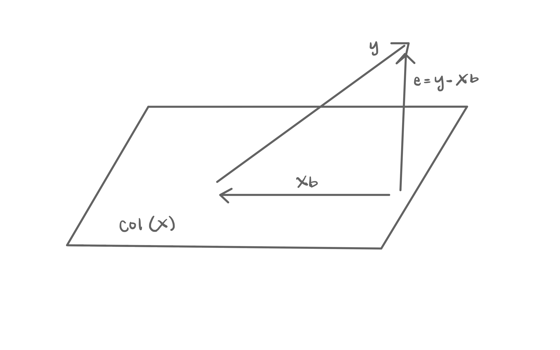
Let $\text{Col}(\mathbf{X})$ be the column space of the design matrix $\mathbf{X}$, the set all possible linear combinations of the columns of $\mathbf{X}$.¹ We cannot derive the values of $\mathbf{y}$ using only linear combinations of $\mathbf{X}$ (recall the error term $\mathit{ϵ}$ in Equation A.12). Therefore, $\mathbf{y}$ is not in $\text{Col}(\mathbf{X})$. We want to find another vector $\mathbf{Xb}$ in $\text{Col}(\mathbf{X})$ that minimizes the distance to $\mathbf{y}$. We call the vector $\mathbf{Xb}$ a projection of $\mathbf{y}$ onto $\text{Col}(\mathbf{X})$.

For any vector $\mathbf{Xb}$ in $\text{Col}(\mathbf{X})$, the vector $\mathbf{e}=\mathbf{y}-\mathbf{Xb}$ is the difference between $\mathbf{y}$ and the projection $\mathbf{Xb}$. We know $\mathbf{X}$ and $\mathbf{y}$ from the data, so we need to find $\mathbf{b}$ that minimizes the length of $\mathbf{e}=\mathbf{y}-\mathbf{Xb}$. It is minimized when $\mathbf{e}$ is orthogonal (also called normal) to $\text{Col}(\mathbf{X})$.

If $\mathbf{A}$, an $n\times k$ matrix, is orthogonal to an $n\times 1$ vector $\mathbf{c}$, then ${\mathbf{A}}^{\mathsf{T}}\mathbf{c}=\mathbf{0}$

Because $\mathbf{e}$ is orthogonal to $\text{Col}(\mathbf{X})$, then ${\mathbf{X}}^{\mathsf{T}}\mathbf{e}=\mathbf{0}$. We plug in $\mathbf{e}=\mathbf{y}-\mathbf{Xb}$ and solve for $\mathbf{b}$.

$$\begin{array}{}\text{(A.22)}& \begin{array}{rl}& {\mathbf{X}}^{\mathsf{T}}(\mathbf{y}-\mathbf{Xb})=\mathbf{0}\\ \Rightarrow & {\mathbf{X}}^{\mathsf{T}}\mathbf{y}-{\mathbf{X}}^{\mathsf{T}}\mathbf{X}\mathbf{b}=0\\ \Rightarrow & {\mathbf{X}}^{\mathsf{T}}\mathbf{y}={\mathbf{X}}^{\mathsf{T}}\mathbf{X}\mathbf{b}\\ \Rightarrow & ({\mathbf{X}}^{\mathsf{T}}\mathbf{X}{)}^{-1}{\mathbf{X}}^{\mathsf{T}}\mathbf{y}=\mathbf{b}\end{array}\end{array}$$

Using the geometric interpretation of least-squares regression, we found that the vector $\mathbf{b}$ that minimizes $\mathbf{e}=\mathbf{y}-\mathbf{Xb}$ is $\hat{\mathbf{b}}=({\mathbf{X}}^{\mathsf{T}}\mathbf{X}{)}^{-1}{\mathbf{X}}^{\mathsf{T}}\mathbf{y}$. This is equal to the estimator found in Equation A.20.

A.4 Hat matrix

The fitted values of least-squares regression are $\mathbf{y}=\mathbf{X}\hat{\mathit{\beta }}$. Plugging in $\hat{\mathit{\beta }}$ from Equation A.20, we have

$$\begin{array}{}\text{(A.23)}& \hat{\mathbf{y}}=\mathbf{X}\hat{\mathit{\beta }}=\underset{\mathbf{H}}{\underbrace{\mathbf{X}({\mathbf{X}}^{\mathsf{T}}\mathbf{X}{)}^{-1}{\mathbf{X}}^{\mathsf{T}}}}\mathbf{y}\end{array}$$

From Equation A.23, $\mathbf{H}=\mathbf{X}({\mathbf{X}}^{\mathsf{T}}\mathbf{X}{)}^{-1}{\mathbf{X}}^{\mathsf{T}}$ is called the hat matrix. The hat matrix is an $n\times n$ matrix that maps $\mathbf{y}$, the vector of observed responses, onto $\hat{\mathbf{y}}$, the vector of fitted values ($\hat{\mathbf{y}}=\mathbf{Hy}$). More precisely, $\mathbf{H}$ is a projection matrix that projects $\mathbf{y}$ onto the column space $\text{Col}(\mathbf{X})$ (see Section A.3.2). Because $\mathbf{H}$ is a projection matrix, it has the following properties:

• $\mathbf{H}$ is symmetric (${\mathbf{H}}^{\mathsf{T}}=\mathbf{H}$).

• $\mathbf{H}$ is idempotent (${\mathbf{H}}^2=\mathbf{H}$).

• If a vector $\mathbf{v}$ is in $\text{Col}(\mathbf{X})$, then $\mathbf{Hv}=\mathbf{v}$.

• If a vector $\mathbf{v}$ is orthogonal to $\text{Col}(\mathbf{X})$, then $\mathbf{Hv}=\mathbf{0}$.

From Equation A.23, the hat matrix only depends on the design matrix $\mathbf{X}$, i.e., it only depends on the values of the predictors. It does not depend on the vector of responses. The diagonal elements $\mathbf{H}$ are the values of leverage. More specifically, $h_{ii}$ is the leverage for the $i^{th}$ observation. Recall from Section 6.4.2 that in simple linear regression, the leverage is a measure of how far an observation’s value of the predictor is from the average value of the predictor across all observations.

$$\begin{array}{}\text{(A.24)}& h_{ii}=\frac{1}{n}+\frac{(x_i-\overline{x}{)}^2}{\sum _{j=1}^n(x_j-\overline{x}{)}^2}\end{array}$$

In multiple linear regression, the leverage is a measure of how far the $i^{th}$ observation is from the center of the $x$ space. It is computed as

$$\begin{array}{}\text{(A.25)}& h_{ii}={\mathbf{x}}_i^{\mathsf{T}}({\mathbf{X}}^{\mathsf{T}}\mathbf{X}{)}^{-1}{\mathbf{x}}_i\end{array}$$

where ${\mathbf{x}}_i^{\mathsf{T}}$ is the $i^{th}$ row of the design matrix $\mathbf{X}$.²

The sum of the leverages for all observation $p+1$ where $p$ is the number of predictors in the model. Thus, $\text{rank}(\mathbf{H})=\sum _{i=1}^n{h}_{ii}=p+1$. The average value of leverage is $\overline{h}=\frac{p+1}{n}$. Observations with leverage greater than $2\overline{h}$ are considered to have large leverage.

Using $\mathbf{H}$, we can write the residuals as

$$\begin{array}{}\text{(A.26)}& \mathbf{e}=\mathbf{y}-\hat{\mathbf{y}}=\mathbf{y}-\mathbf{Hy}=(\mathbf{I}-\mathbf{H})\mathbf{y}\end{array}$$

Equation A.26 shows one feature of observations with large leverage. Observations with large leverage tend to have small residuals. In other words, the model tends to pull towards observations with large leverage.

A.5 Assumptions of linear regression

In Section 5.3, we introduced four assumptions of linear regression. Given the matrix form of the linear regression on model in Equation A.12, $\mathbf{y}=\mathbf{X}\mathit{\beta }+\mathit{ϵ}$ such that $\mathit{ϵ}\sim N(\mathbf{0},{\sigma }_{ϵ}^2\mathbf{I})$ , these assumptions are the following:

1. The distribution of the response $\mathbf{y}$ given $\mathbf{X}$ is normal.
2. The expected value of $\mathbf{y}$ is $\mathbf{X}\mathit{\beta }$. There is a linear relationship between the response and predictor variables.
3. The variance $\mathbf{y}$ given $\mathbf{X}$ is ${\sigma }_{ϵ}^2\mathbf{I}$.
4. The error terms in $\mathit{ϵ}$ are independent. This also means the observations are independent of one another.

From these assumptions, we write the distribution of $\mathbf{y}$ given the regression model in Equation A.27.

$$\begin{array}{}\text{(A.27)}& \mathbf{y}|\mathbf{X}\sim N(\mathbf{X}\mathit{\beta },{\sigma }_{ϵ}^2\mathbf{I})\end{array}$$

In Section A.2, we showed Assumption 4 from the distribution of the error terms. Here we will show Assumptions 1 - 3.

Suppose $\mathbf{z}$ is a (multivariate) normal random variable such that $\mathbf{z}\sim N(\mathit{\mu },\mathbf{\Sigma })$. A linear transformation of $\mathbf{z}$ is also multivariate normal, such that

$$\mathbf{A}\mathbf{z}+\mathbf{B}\sim N(\mathbf{A}\mathit{\mu }+\mathbf{B},\mathbf{A}\mathbf{\Sigma }{\mathbf{A}}^{\mathsf{T}})$$

The distribution of the error terms $\mathit{ϵ}$ is normal, and the vector of responses $\mathbf{y}$ is linear combination of the error terms. More specifically, $\mathbf{y}$ is computed as the error terms, shifted by $\mathbf{X}\mathit{\beta }$. Thus, from the math property above, we know that $\mathbf{y}$ is normally distributed.

Expected value of a vector

Let $\mathbf{z}={\left[\begin{array}{ccc}{z}_1& \dots & z_p\end{array}\right]}^{\mathsf{T}}$ be a $p\times 1$ vector of random variables. Then $E(\mathbf{z})=E{\left[\begin{array}{ccc}{z}_1& \dots & z_p\end{array}\right]}^{\mathsf{T}}={\left[\begin{array}{ccc}E(z_1)& \dots & E(z_p)\end{array}\right]}^{\mathsf{T}}$

Let $\mathbf{A}$ be an $n\times p$ matrix of constants, $\mathbf{C}$ a $n\times 1$ vector of random variables, and $\mathbf{z}$ a $p\times 1$ vector of random variables. Then

$$E(\mathbf{Az}+\mathbf{C})=\mathbf{A}E(\mathbf{z})+E(\mathbf{C})$$

Next, let’s show Assumption 2 that the expected value of $\mathbf{y}=\mathbf{X}\mathit{\beta }$ in linear regression. We can get the expected value of $\mathbf{y}$ from the mathematical properties above used for Assumption 1. Here, we show Assumption 2 directly from the properties of expected values.

$$\begin{array}{}\text{(A.28)}& \begin{array}{rl}E(\mathbf{y})& =E(\mathbf{X}\mathit{\beta }+\mathit{ϵ})\\ & =E(\mathbf{X}\mathit{\beta })+E(\mathit{ϵ})\\ & =\mathbf{X}\mathit{\beta }+\mathbf{0}\\ & =\mathbf{X}\mathit{\beta }\end{array}\end{array}$$

Let $\mathbf{z}$ be a $p\times 1$ vector of random variables. Then

$$Var(\mathbf{z})=E[(\mathbf{z}-E(\mathbf{z}))(\mathbf{z}-E(\mathbf{z}){)}^{\mathsf{T}}]$$

Lastly, we show Assumption 3 that $Var(\mathbf{y})={\sigma }_{ϵ}^2\mathbf{I}$ in linear regression. Similar to the expected value, we can get the variance from the mathematical property used to show Assumption 1. Here, we show Assumption 3 directly from the properties of variance. $$\begin{array}{}\text{(A.29)}& \begin{array}{rl}Var(\mathbf{y})& =E[(\mathbf{y}-E(\mathbf{y}))(\mathbf{y}-E(\mathbf{y}){)}^{\mathsf{T}}]\\ & =E[(\mathbf{X}\mathit{\beta }+\mathit{ϵ}-\mathbf{X}\mathit{\beta })(\mathbf{X}\mathit{\beta }+\mathit{ϵ}-\mathbf{X}\mathit{\beta }{)}^{\mathsf{T}}]\\ & =E[\mathit{ϵ}{\mathit{ϵ}}^{\mathsf{T}}]\\ (\text{given }E(\mathit{ϵ}=\mathbf{0}))& =E[(\mathit{ϵ}-E(\mathit{ϵ}))(\mathit{ϵ}-E(\mathit{ϵ}){)}^{\mathsf{T}}]\\ & =Var(\mathit{ϵ})\\ & ={\sigma }_{ϵ}^2\mathbf{I}\end{array}\end{array}$$

A.6 Distribution of model coefficients

In Section 8.4.1, we introduced the distribution of a model coefficient ${\hat{\beta }}_j\sim N({\beta }_j,S{E}_{{\hat{\beta }}_j}^2)$. In matrix notation, the distribution of all the estimated coefficients $\hat{\mathit{\beta }}$ is

$$\begin{array}{}\text{(A.30)}& \hat{\mathit{\beta }}\sim N(\mathit{\beta },{\sigma }_{ϵ}^2({\mathbf{X}}^{\mathsf{T}},\mathbf{X}{)}^{-1})\end{array}$$

Similar to Section A.5, let’s derive each part of this distribution. We’ll start with $E(\hat{\mathit{\beta }})=\mathit{\beta }$.

$$\begin{array}{}\text{(A.31)}& \begin{array}{rl}E(\hat{\mathit{\beta }})& =E(({\mathbf{X}}^{\mathsf{T}}\mathbf{X}{)}^{-1}{\mathbf{X}}^{\mathsf{T}}\mathbf{y})\\ & =({\mathbf{X}}^{\mathsf{T}}\mathbf{X}{)}^{-1}{\mathbf{X}}^{\mathsf{T}}E(\mathbf{y})\\ & =({\mathbf{X}}^{\mathsf{T}}\mathbf{X}{)}^{-1}{\mathbf{X}}^{\mathsf{T}}E(\mathbf{X}\mathit{\beta }+\mathit{ϵ})\\ & =({\mathbf{X}}^{\mathsf{T}}\mathbf{X}{)}^{-1}{\mathbf{X}}^{\mathsf{T}}E(\mathbf{X}\mathit{\beta })+({\mathbf{X}}^{\mathsf{T}}\mathbf{X}{)}^{-1}{\mathbf{X}}^{\mathsf{T}}E(\mathit{ϵ})\\ & =({\mathbf{X}}^{\mathsf{T}}\mathbf{X}{)}^{-1}{\mathbf{X}}^{\mathsf{T}}\mathbf{X}\mathit{\beta }+\mathbf{0}\\ & =\mathit{\beta }\end{array}\end{array}$$

Next, we show that $Var(\hat{\mathit{\beta }})={\sigma }_{ϵ}^2\mathbf{I}$.

$$\begin{array}{}\text{(A.32)}& \begin{array}{rl}Var(\hat{\mathit{\beta }})& =E[(\hat{\mathit{\beta }}-E(\hat{\mathit{\beta }}))(\hat{\mathit{\beta }}-E(\hat{\mathit{\beta }}){)}^{\mathsf{T}}]\\ & =E[(({\mathbf{X}}^{\mathsf{T}}\mathbf{X}{)}^{-1}{\mathbf{X}}^{\mathsf{T}}\mathbf{y}-\mathit{\beta })(({\mathbf{X}}^{\mathsf{T}}\mathbf{X}{)}^{-1}{\mathbf{X}}^{\mathsf{T}}\mathbf{y}-\mathit{\beta }{)}^{\mathsf{T}}]\\ & =E[(({\mathbf{X}}^{\mathsf{T}}\mathbf{X}{)}^{-1}{\mathbf{X}}^{\mathsf{T}}(\mathbf{X}\mathit{\beta }+\mathit{ϵ})-\mathit{\beta })(({\mathbf{X}}^{\mathsf{T}}\mathbf{X}{)}^{-1}{\mathbf{X}}^{\mathsf{T}}(\mathbf{X}\mathit{\beta }+\mathit{ϵ})-\mathit{\beta }{)}^{\mathsf{T}}]\\ & \dots \text{After distributing and simplifying}\dots \\ & =E[({\mathbf{X}}^{\mathsf{T}}\mathbf{X}{)}^{-1}{\mathbf{X}}^{\mathsf{T}}\mathit{ϵ}{\mathit{ϵ}}^{\mathsf{T}}\mathbf{X}({\mathbf{X}}^{\mathsf{T}}\mathbf{X}{)}^{-1}]\\ & =({\mathbf{X}}^{\mathsf{T}}\mathbf{X}{)}^{-1}{\mathbf{X}}^{\mathsf{T}}\underset{{\sigma }_{ϵ}^2\mathbf{I}}{\underbrace{E(\mathit{ϵ}{\mathit{ϵ}}^{\mathsf{T}})}}\mathbf{X}({\mathbf{X}}^{\mathsf{T}}\mathbf{X}{)}^{-1}\\ & ={\sigma }^2\mathbf{I}({\mathbf{X}}^{\mathsf{T}}\mathbf{X}{)}^{-1}{\mathbf{X}}^{\mathsf{T}}\mathbf{X}({\mathbf{X}}^{\mathsf{T}}\mathbf{X}{)}^{-1}\\ & ={\sigma }_{ϵ}^2({\mathbf{X}}^{\mathsf{T}}\mathbf{X}{)}^{-1}\end{array}\end{array}$$

Lastly, we show that the distribution of $\mathit{\beta }$ is normal. We’ll start by rewriting $\hat{\mathit{\beta }}$ in terms of $\mathit{\beta }$.

$$\begin{array}{}\text{(A.33)}& \begin{array}{rl}\hat{\mathit{\beta }}& =({\mathbf{X}}^{\mathsf{T}}\mathbf{X}{)}^{-1}{\mathbf{X}}^{\mathsf{T}}\mathbf{y}\\ & =({\mathbf{X}}^{\mathsf{T}}\mathbf{X}{)}^{-1}{\mathbf{X}}^{\mathsf{T}}(\mathbf{X}\mathit{\beta }+\mathit{ϵ})\\ & =\mathit{\beta }+({\mathbf{X}}^{\mathsf{T}}\mathbf{X}{)}^{-1}{\mathbf{X}}^{\mathsf{T}}\mathit{ϵ}\end{array}\end{array}$$

From Equation A.33, we see that $\hat{\mathit{\beta }}$ is a linear combination of the error terms $\mathit{ϵ}$. From the math property in Section A.5, because $\mathit{ϵ}$ is normally distributed, the linear combination is also normally distributed. Thus, the distribution of the coefficients $\hat{\mathit{\beta }}$ is normal.

A.7 Multicollinearity

Recall the design matrix for a linear regression model with $p$ predictors in Equation A.13

$$\begin{array}{}\text{(A.34)}& \mathbf{X}=\left[\begin{array}{cccc}1& x_{11}& \dots & x_{1p}\\ ⋮& ⋮& \ddots & ⋮\\ 1& x_{n1}& \dots & x_{np}\end{array}\right]\end{array}$$

The design matrix $\mathbf{X}$ has full column rank $\text{rank}(\mathbf{X})=(p+1)$ in linear regression. This means there are no linear dependencies among the columns, and thus no column is a perfect linear combination of the others. The equation for the least-squares estimator $\hat{\mathit{\beta }}$ in Equation A.20 includes the term $({\mathbf{X}}^{\mathsf{T}}\mathbf{X}{)}^{-1}$. If $\mathbf{X}$ is not full rank, then ${\mathbf{X}}^{\mathsf{T}}\mathbf{X}$ is not full rank, and is therefore singular (not invertible). Thus, if there are linear dependencies in $\mathbf{X}$, we are unable to compute an the least-squares estimator $\hat{\mathit{\beta }}$.

Let ${\mathbf{x}}_1,{\mathbf{x}}_2,\dots ,{\mathbf{x}}_p$ be a sequence of vectors. Then, ${\mathbf{x}}_1,{\mathbf{x}}_2,\dots ,{\mathbf{x}}_p$ are linearly dependent, if there exists scalars $a_1,a_2,\dots ,a_p$ such that

$$a_1{\mathbf{x}}_1+a_2{\mathbf{x}}_2+\cdots +a_p{\mathbf{x}}_p=\mathbf{0}$$

where $a_1,a_2,\dots ,a_p$ are not all 0.

In practice, we rarely have perfect linear dependencies. In fact, this is mathematically why we only include $k-1$ terms in the model for a categorical predictor with $k$ levels. Ideally the columns of $\mathbf{X}$ would be orthogonal, indicating the predictors are completely independent on one another. In practice, we expect there to be some dependence between predictors (we see this from the non-zero off diagonals in $Var(\hat{\mathit{\beta }})$). If two or more variables are highly correlated, then there will be near linear dependence in the columns. This near-linear dependence is called multicollinearity.

In Section 8.6 we discussed the practical issues that come from the presence of multicollinearity. These primarily stem from the fact that when there is multicollinearity, ${\mathbf{X}}^{\mathsf{T}}\mathbf{X}$ is near-singular (almost a singular matrix) to a, thus making $({\mathbf{X}}^{\mathsf{T}}\mathbf{X}{)}^{-1}$ very large and unstable. Consequently, $Var(\hat{\mathit{\beta }})$ is then large and unstable, thus making hard to find stable values for the least-squares estimators.

A.8 Maximum Likelihood Estimation

In Section 10.2.3, we introduced the likelihood function to understand the model performance statistics AIC and BIC. We also used a likelihood function to estimate the coefficients in logistic regression (more on this in Appendix B). The likelihood function is a measure of how likely it is we observe our data given particular value(s) of model parameters. When working with likelihood functions, we have fixed data (our observed sample data) and we can try out different values for the model parameters ($\mathit{\beta }$ and ${\sigma }_{ϵ}^2$ in the context of regression).³

Let $\mathbf{z}$ be a $p\times 1$ vector of random variables, such that $\mathbf{z}$ follows a multivariate normal distribution with mean $\mathit{\mu }$ and variance $\mathbf{\Sigma }$. Then the probability density function of $\mathbf{z}$ is

$$f(\mathbf{z})=\frac{1}{(2\pi {)}^{p/2}|\mathbf{\Sigma }{|}^{1/2}}\exp \{-\frac{1}{2}(\mathbf{z}-\mathit{\mu }{)}^{\mathsf{T}}{\mathbf{\Sigma }}^{-1}(\mathbf{z}-\mathit{\mu })\}$$

In Section A.5, we showed that the vector of responses $\mathbf{y}$ can be written as $\mathbf{y}|\mathbf{X}\sim N(\mathbf{X}\mathit{\beta },{\sigma }_{ϵ}^2\mathbf{I})$. Using this distribution to describe the relationship between the response and predictor variables, the likelihood function for the regression parameters $\mathit{\beta }$ and ${\sigma }_{ϵ}^2$ is

$$\begin{array}{}\text{(A.35)}& L(\mathit{\beta },{\sigma }_{ϵ}^2|\mathbf{X},\mathbf{y})=\frac{1}{(2\pi {)}^{n/2}{\sigma }_{ϵ}^n}\exp \{-\frac{1}{2{\sigma }_{ϵ}^2}(\mathbf{y}-\mathbf{X}\mathit{\beta }{)}^{\mathsf{T}}(\mathbf{y}-\mathbf{X}\mathit{\beta })\}\end{array}$$

where $n$ is the number of observations, the mean is $\mathbf{X}\mathit{\beta }$ and the variance is ${\sigma }_{ϵ}^2\mathbf{I}$.

The data $\mathbf{y}$ and $\mathbf{X}$ are fixed (we use the same sample data in the analysis!), so we can plug in values for $\mathit{\beta }$ and ${\sigma }_{ϵ}^2$ to determine the likelihood of obtaining those values for the parameters given the observed data. In Section A.3.1, we used least-squares estimation (minimizing $SSR$ ) find the estimated coefficients $\hat{\mathit{\beta }}$. Another approach to estimate $\mathit{\beta }$ (and ${\sigma }_{ϵ}^2$) is to find $\hat{\mathit{\beta }}$ (and ${\hat{\sigma }}_{ϵ}^2$) that maximizes the likelihood function in Equation A.35. This is called maximum likelihood estimation.

To make the calculations more manageable, instead of maximizing the likelihood function, we will instead maximize its logarithm, i.e. the log-likelihood function. The values of the parameters that maximize the log-likelihood function are those that maximize the likelihood function. The log-likelihood function is

$$\begin{array}{}\text{(A.36)}& \begin{array}{rl}\log L(\mathit{\beta },{\sigma }_{ϵ}^2& |\mathbf{X},\mathbf{y})\\ & =-\frac{n}{2}\log (2\pi )-n\log ({\sigma }_{ϵ})-\frac{1}{2{\sigma }_{ϵ}^2}(\mathbf{y}-\mathbf{X}\mathit{\beta }{)}^{\mathsf{T}}(\mathbf{y}-\mathbf{X}\mathit{\beta })\end{array}\end{array}$$

Given a fixed value of ${\sigma }_{ϵ}^2$, the log-likelihood in Equation A.36 is maximized when $(\mathbf{y}-\mathbf{X}\mathit{\beta }{)}^{\mathsf{T}}(\mathbf{y}-\mathbf{X}\mathit{\beta })$ is minimized. This is equivalent to minimizing the $SSR$ in Equation A.15. Thus, the least-squares estimator of $\mathit{\beta }$ is also the maximum likelihood estimator ( $\hat{\beta }=({\mathbf{X}}^{\mathsf{T}}\mathbf{X}{)}^{-1}{\mathbf{X}}^{\mathsf{T}}\mathbf{y}$) when the error terms are defined as in Equation A.12.

We previously found $\hat{\mathit{\beta }}$ using least-squares estimation and the geometry of regression in Section A.3.1, so why does it matter that $\hat{\mathit{\beta }}$ is also the maximum likelihood estimator? First, maximum likelihood estimation is used to find the coefficients for generalized linear models and many other statistical models that go beyond linear regression (we’ll see how its used for logistic regression in Appendix B). In fact, Casella and Berger (2024) stated maximum likelihood estimation is “by far, the most popular technique for deriving estimators.” [pp. 315]. Second, maximum likelihood estimators have nice statistical properties. These properties are beyond the scope of this text, but we refer interested readers to Chapter 7 of Casella and Berger (2024) for an in-depth discussion of maximum likelihood estimators and their properties.

A.9 Variable transformations

In Chapter 9, we introduced regression models with transformations on the response and/or predictor variables. Here we will share some of the mathematical details behind the interpretation of the coefficients in these models.

A.9.1 Transformation on the response variable

In Section 9.2, we introduced a linear regression model with a log transformation on the response variable

$$\begin{array}{}\text{(A.37)}& \log (Y)={\beta }_0+{\beta }_1{X}_1+\cdots +{\beta }_p{X}_p+ϵ\end{array}$$

In this text, $\log (a)$ is the natural log of $a$ (also denoted as $\ln (a)$).

• $\log (a)+\log (b)=\log (ab)$.

• $\log (a)-\log (b)=\log (\frac{a}{b})$

• $e^{\log (a)}=a$

• $e^{b\log (a)}=a^b$

From Chapter 7, we have that the change in $\log (Y)$ when $X_j$ increase by 1 unit is ${\beta }_j$. Thus ${\beta }_j=\log (Y|X_j+1)-\log (Y|X_j)$, where $Y|X_j+1$ is the value of $Y$ when we plug in $X_j+1$ and $Y|X_j$ is the value of $Y$ when we plug in $X_j$. In practice, we interpret the model coefficients ${\beta }_j$ in terms of the original variable $Y$, so we can use the rules of logarithms and exponents to rewrite this in terms of the original units of the response variable.

$$\begin{array}{rl}{\beta }_j& =\log (Y|X_j+1)-\log (Y|X_j)\\ & =\log (\frac{Y|X_j+1}{Y|X_j})\\ \Rightarrow {\beta }_j\times Y|X_j& =Y|X_j+1\end{array}$$

Thus given the model in Equation A.37, when $X_j$ increases by 1 unit, we expect $Y$ to multiply by ${\beta }_j$, assuming all other predictors are held constant.

A.9.2 Transformation on predictor variable(s)

Next, we consider the models introduced in Section 9.3 that have a log transformation on a predictor variable.

$$\begin{array}{}\text{(A.38)}& Y={\beta }_0+{\beta }_1{X}_1+\cdots +{\beta }_j\log (X_j)+\cdots +{\beta }_p{X}_p+ϵ\end{array}$$

Now, we because the predictor $X_j$ has been transformed to the logarithmic scale, we write interpretations in terms of a multiplicative change in $X_j$. More specifically, given a constant $C$, $\log (C{X}_j)=\log (C)+\log (X_j)$. Let $Y|C{X}_j$ be the expected value of $Y$ when we plug in $C{X}_j$ and $Y|X_j$ be the expected value of $Y$ when we plug in $X_j$. Assuming all other predictors held constant, we have

$$\begin{array}{rl}Y|C{X}_j-Y|CX& ={\beta }_j\log (C{X}_j)-{\beta }_j\log (X_j)\\ & ={\beta }_j[\log (C{X}_j)-\log (X_j)\\ & ={\beta }_j[\log (C)+\log (X_j)-\log (X_j)]\\ & ={\beta }_j\log (C)\\ \Rightarrow Y|C{X}_j& =Y|X_j+{\beta }_j\log (C)\end{array}$$

Thus, given the model in Equation A.38, when predictor $X_j$ is multiplied by a constant $C$, we expect $Y$ to change (increase or decrease) by ${\beta }_j\log (C)$, holding all other predictors constant.

A.9.3 Transformation on response and predictor variables

Lastly, we show the mathematics behind the interpretation of a model coefficient ${\beta }_j$ for the linear regression models introduced in Section 9.4 with a log transformation on the response variable and a predictor variable. As in Section A.9.1, we want to write the interpretation in terms of the original response variable $Y$.

$$\begin{array}{}\text{(A.39)}& \log (Y)={\beta }_0+{\beta }_1{X}_1+\cdots +{\beta }_j\log (X_j)+\cdots +{\beta }_p{X}_p\end{array}$$

Combining the results from Section A.9.1 and Section A.9.2 and holding all other predictors constant, we have

$$\begin{array}{}\text{(A.40)}& \begin{array}{rl}\log (Y|C{X}_j)-\log (Y|X_j)& ={\beta }_j\log (C)\\ \log (\frac{Y|C{X}_j}{Y|X_j})& ={\beta }_j\log (C)\\ \frac{Y|C{X}_j}{Y|X_j}& =C^{{\beta }_j}\\ \Rightarrow Y|C{X}_j& =Y|X_j{C}^{{\beta }_j}\end{array}\end{array}$$

Therefore, given the model in Equation A.39 with a transformed response variable and transformed predictor, when $X_j$ is multiplied by a constant $C$, why is expected to multiply by $C^{{\beta }_j}$, holding all other predictors constant.

Casella, George, and Roger Berger. 2024. Statistical Inference. 2nd ed. CRC Press.

---

1. This is the span of $\mathbf{X}$.

2. Note that when there is a single predictor, Equation A.24 and Equation A.25 produce the same result.

3. Note that the likelihood function is not the same as a probability function. In a probability function, we fix the model parameters and plug in different values for the data.