
expenditure_m
The analysis in this chapter focuses on the amount of money colleges and universities spend in total on men’s and women’s basketball programs in a single year. The data come from the Equity in Athletics Data Analysis (EADA) tool from the Office of Postsecondary Education in the United States Department of Education (ope.ed.gov/athletics). Every college and university in the United States that offers both student financial aid and intercollegiate programs (this includes nearly all colleges and universities) are required by law to submit information about its spending and revenue on athletic programs annually (U.S. Department of Education, Office of Postsecondary Education 2025).
The EADA is a very rich data set with over 300 hundred variables about basketball and all other collegiate sports for all 2-year and 4-year institutions that meet the federal reporting requirements.1 This analysis will focus on data from schools in the National Collegiate Athletics Association (NCAA) Division I. According to the NCAA, Division I institutions are those that “have to sponsor at least seven sports for men and seven for women (or six for men and eight for women) with two team sports for each gender. Each playing season has to be represented by each gender as well. There are contest and participant minimums for each sport, as well as scheduling criteria” (NCAA 2013). We will refer to these institutions as “NCAA Division I colleges” or just “colleges” throughout the remainder of the chapter.
The data in ncaa-basketball-DI-2023-2024.csv contains data from the 2023 - 2024 academic year. We will use the following variables that have been derived from variables in the EADA.
expenditure_m: Total expenditure on basketball programs (in millions of US dollars)enrollment_th: Total student enrollment (in thousands)type: Whether the college is public or privateregion: Region where the college is located. The regions are defined using the state.region vector in R.The goal of this analysis is to use the student enrollment, region, and type of college to explain variability in the total expenditure on basketball programs in the 2023 - 2024 academic year.
expenditure_m
enrollment_th
region
type
enrollment_th and expenditure_m
| Variable | Mean | SD | Min | Q1 | Median (Q2) | Q3 | Max | Missing |
|---|---|---|---|---|---|---|---|---|
| expenditure_m | 8.3 | 7.0 | 1.3 | 3.7 | 5.0 | 10.8 | 38.1 | 0 |
| enrollment_th | 11.9 | 9.9 | 1.0 | 4.6 | 7.9 | 17.8 | 59.6 | 0 |
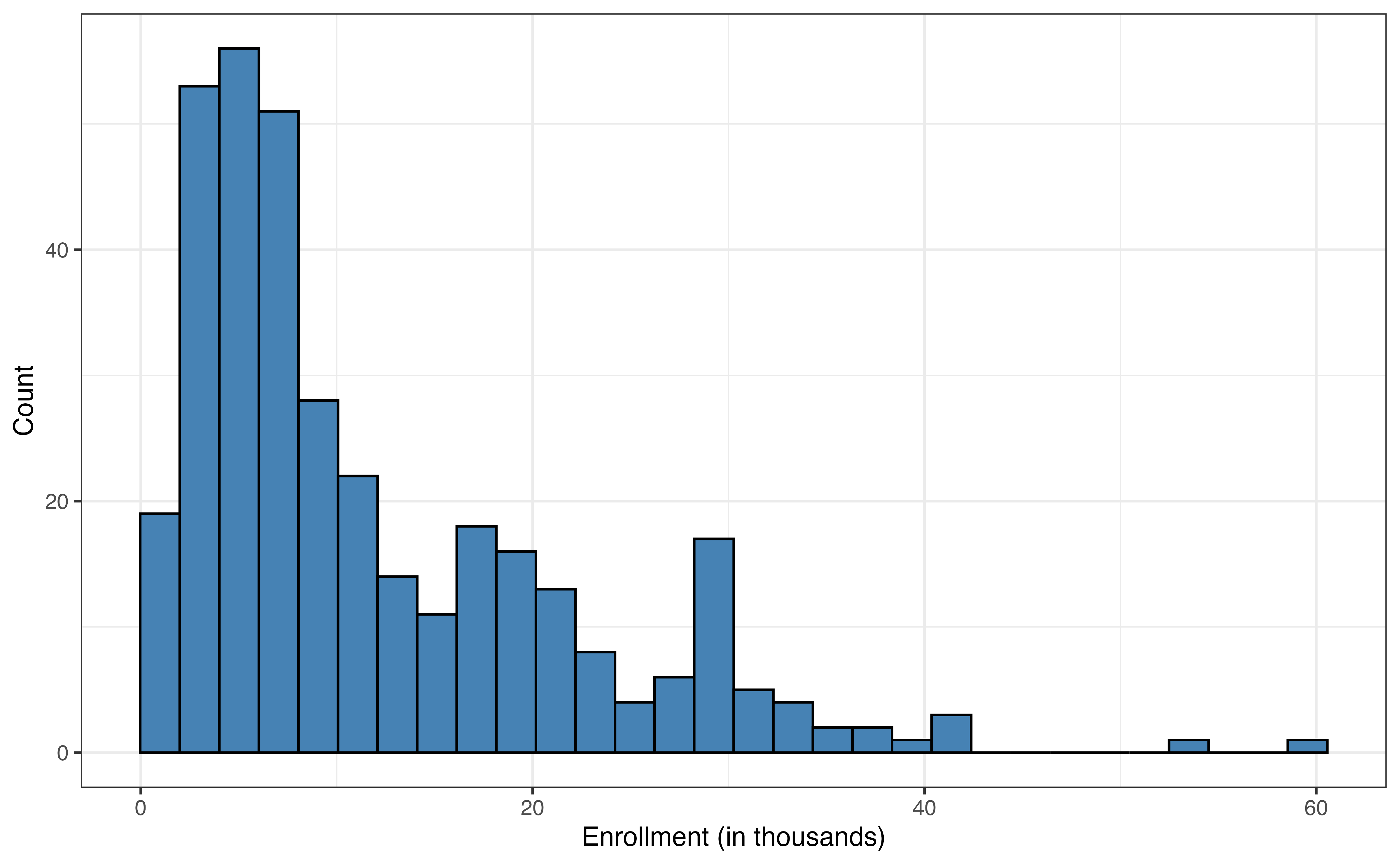
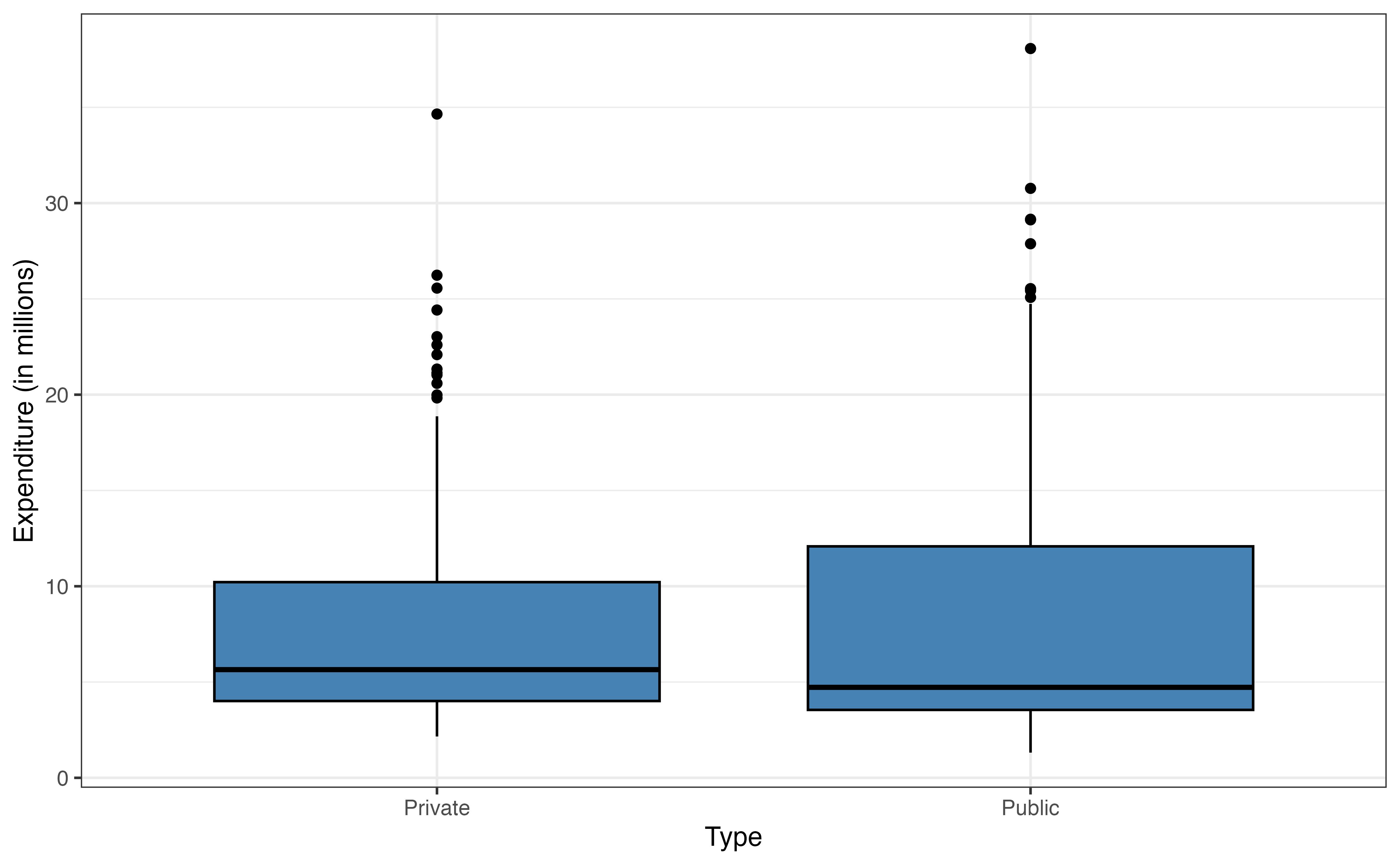
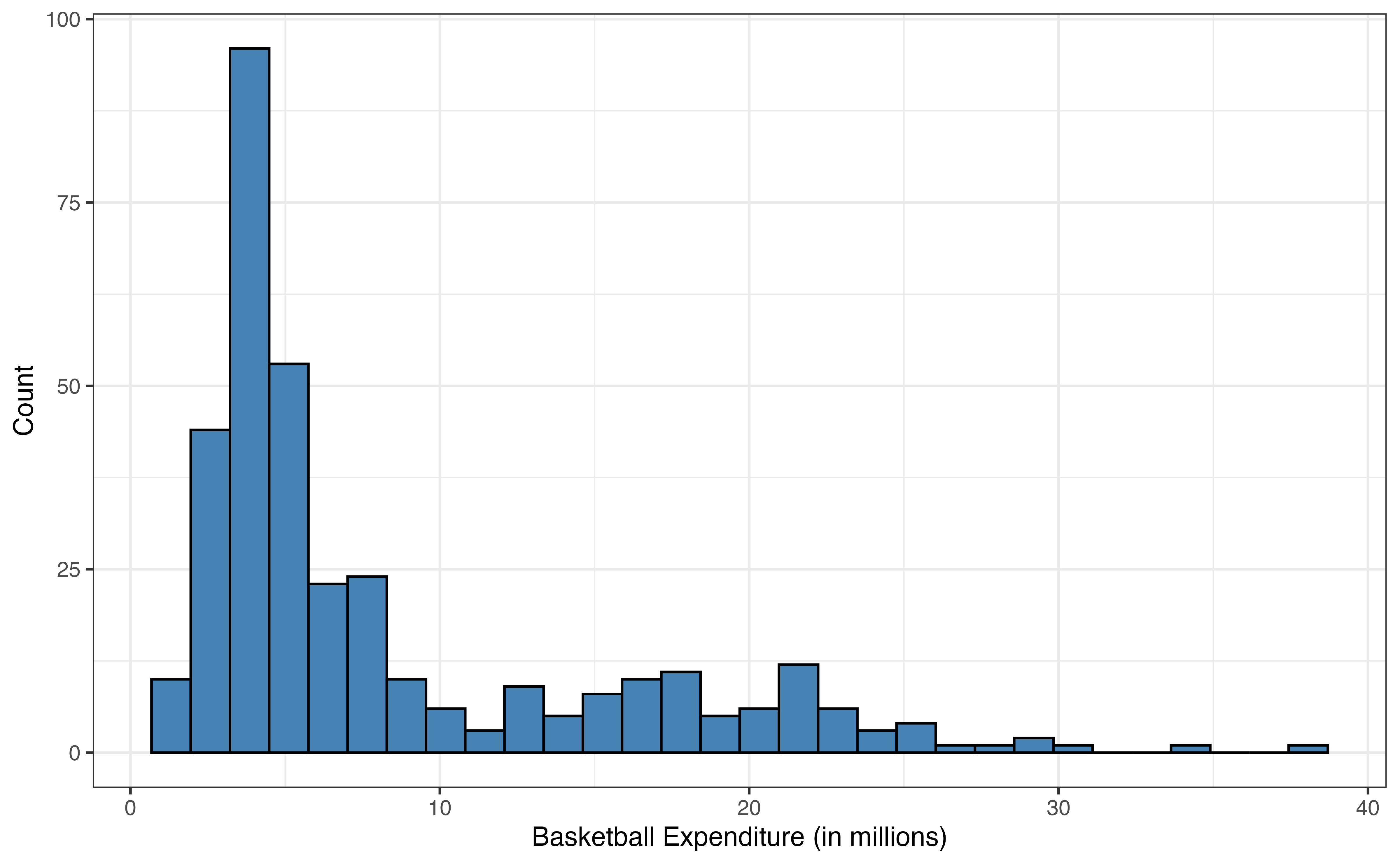
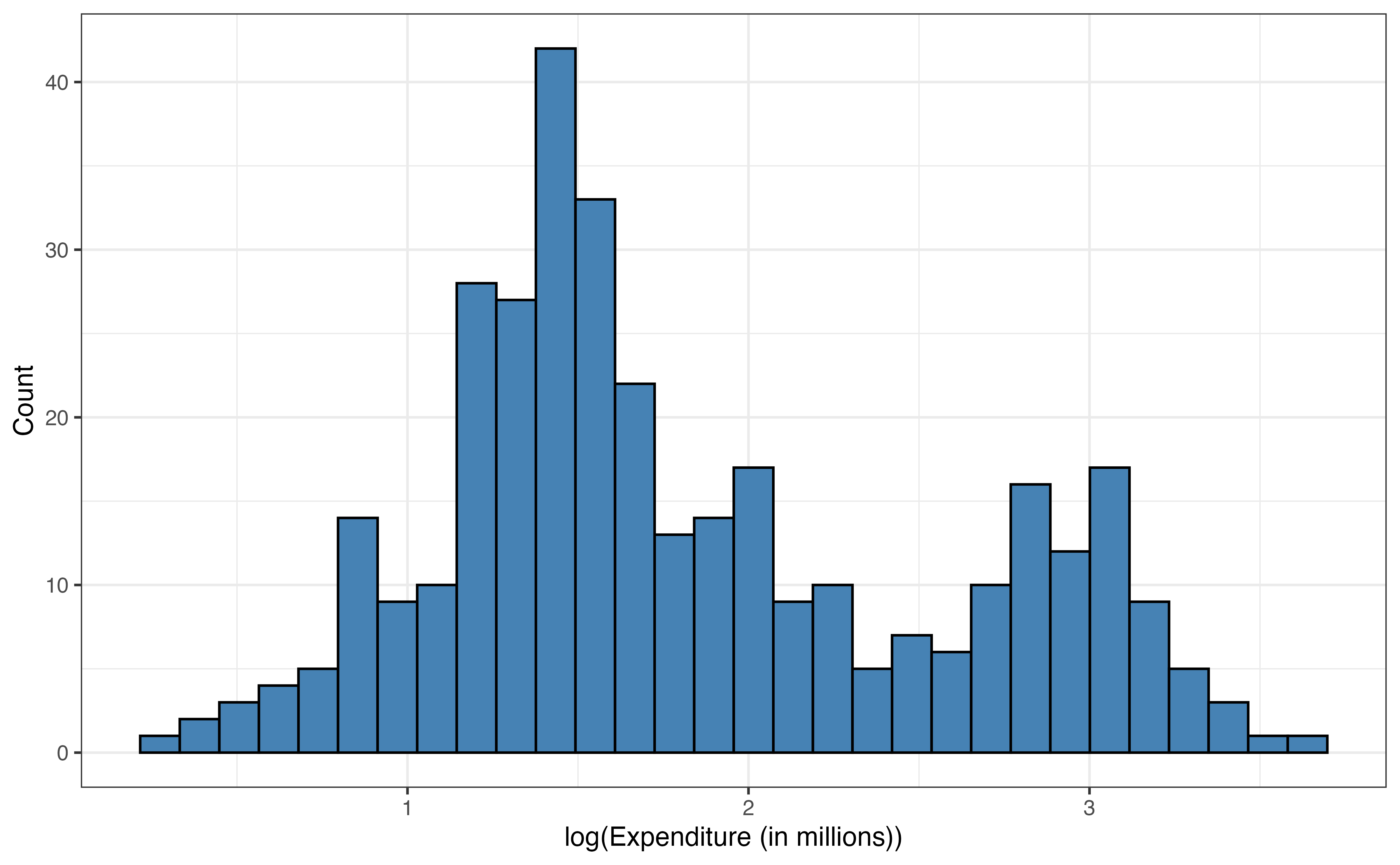
The response variable expenditure_m in Figure 9.1 is unimodal and skewed right. The median expenditure on basketball programs is 5 million dollars, but there are a few colleges that spent over 30 million dollars on basketball programs in 2023 - 2024. Similarly, enrollment_th in Figure 9.2 (a) is unimodal and skewed right, with a median enrollment of about 7900 students. There are some very large colleges in the data set with enrollments of over 40,000 students.
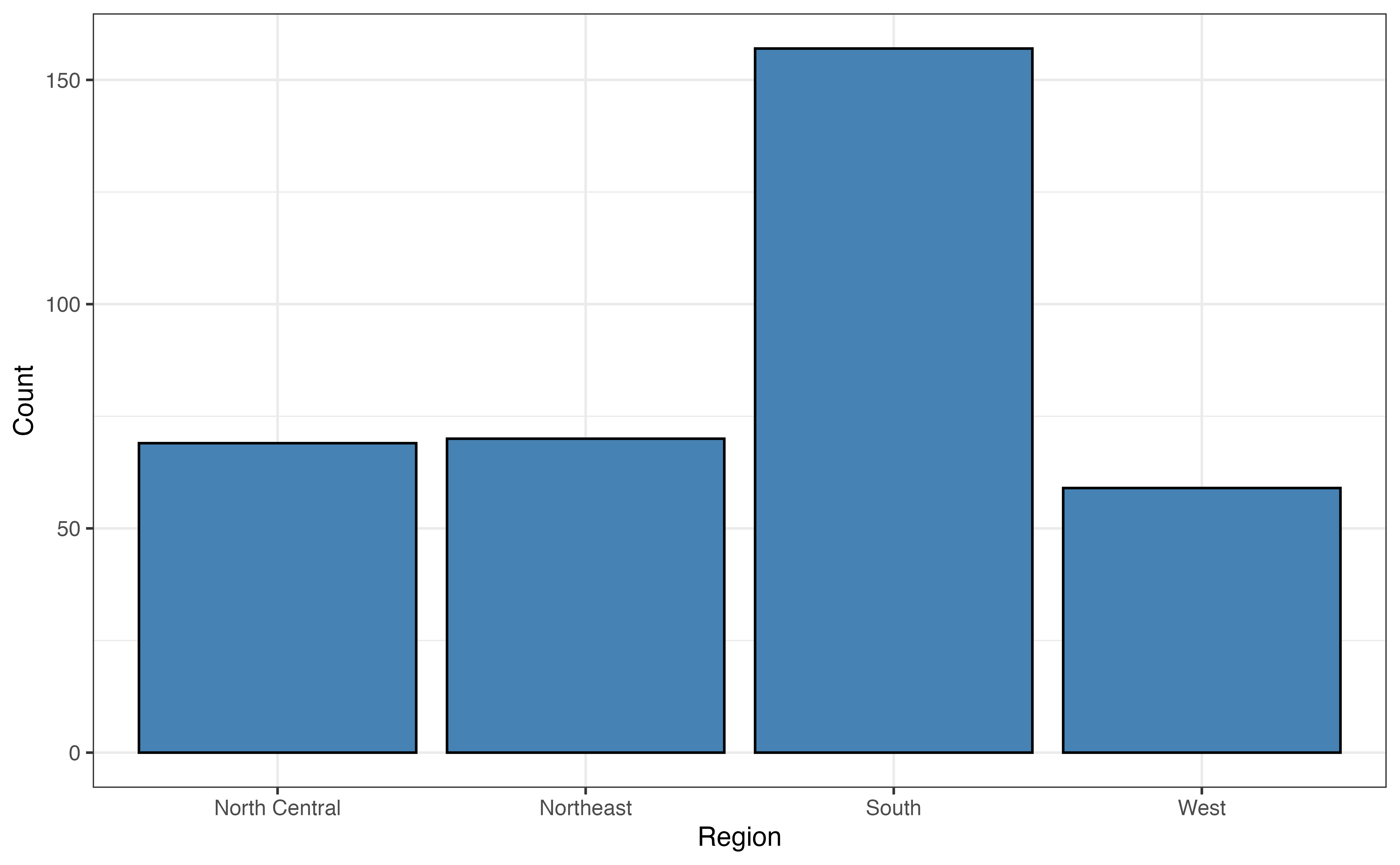
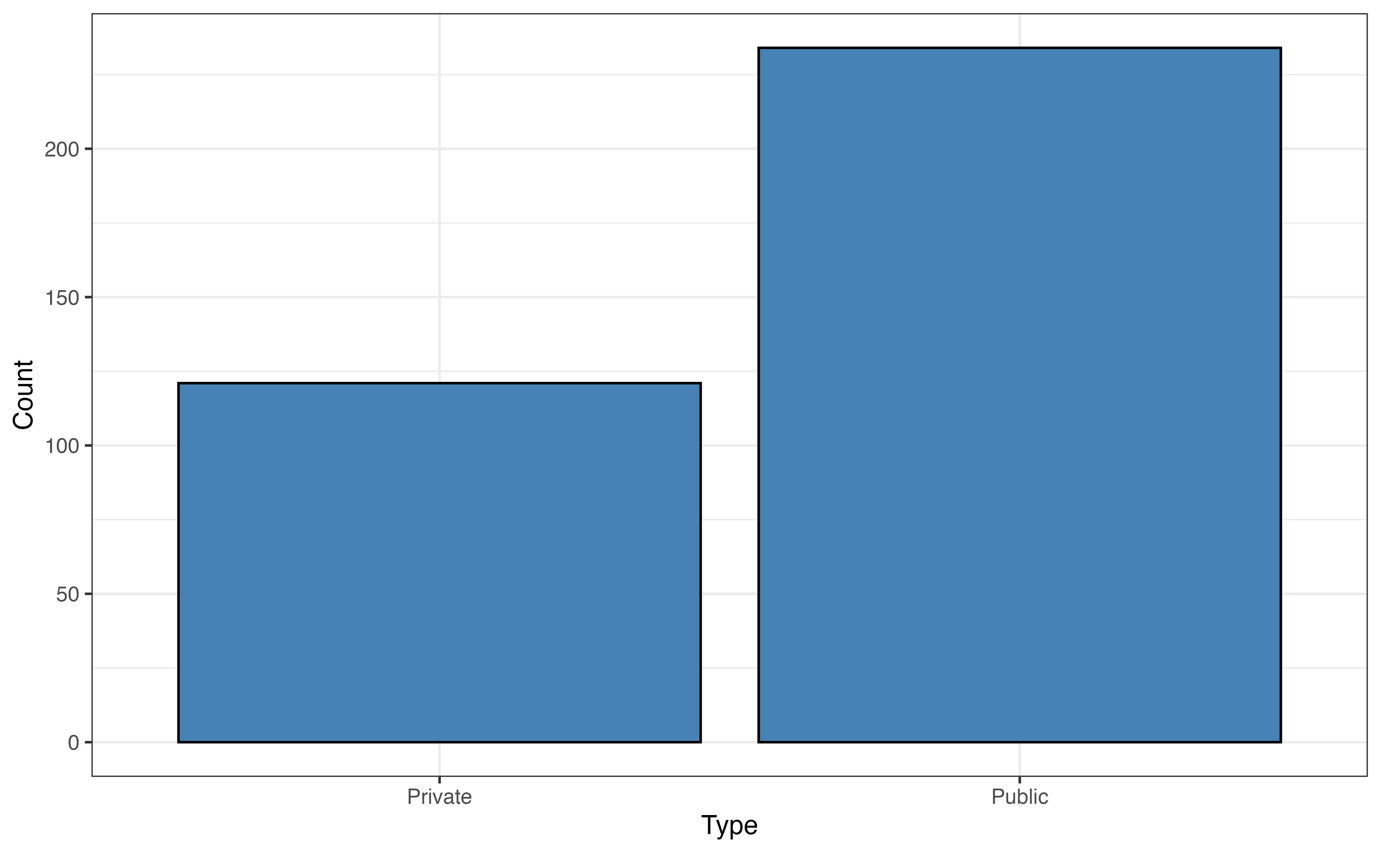
Almost half of the 355 colleges in the data are located in the South region (Figure 9.2 (b)), and about two-thirds of the colleges in the data set are public institutions (Figure 9.2 (c)).

expenditure_m versus enrollment_th
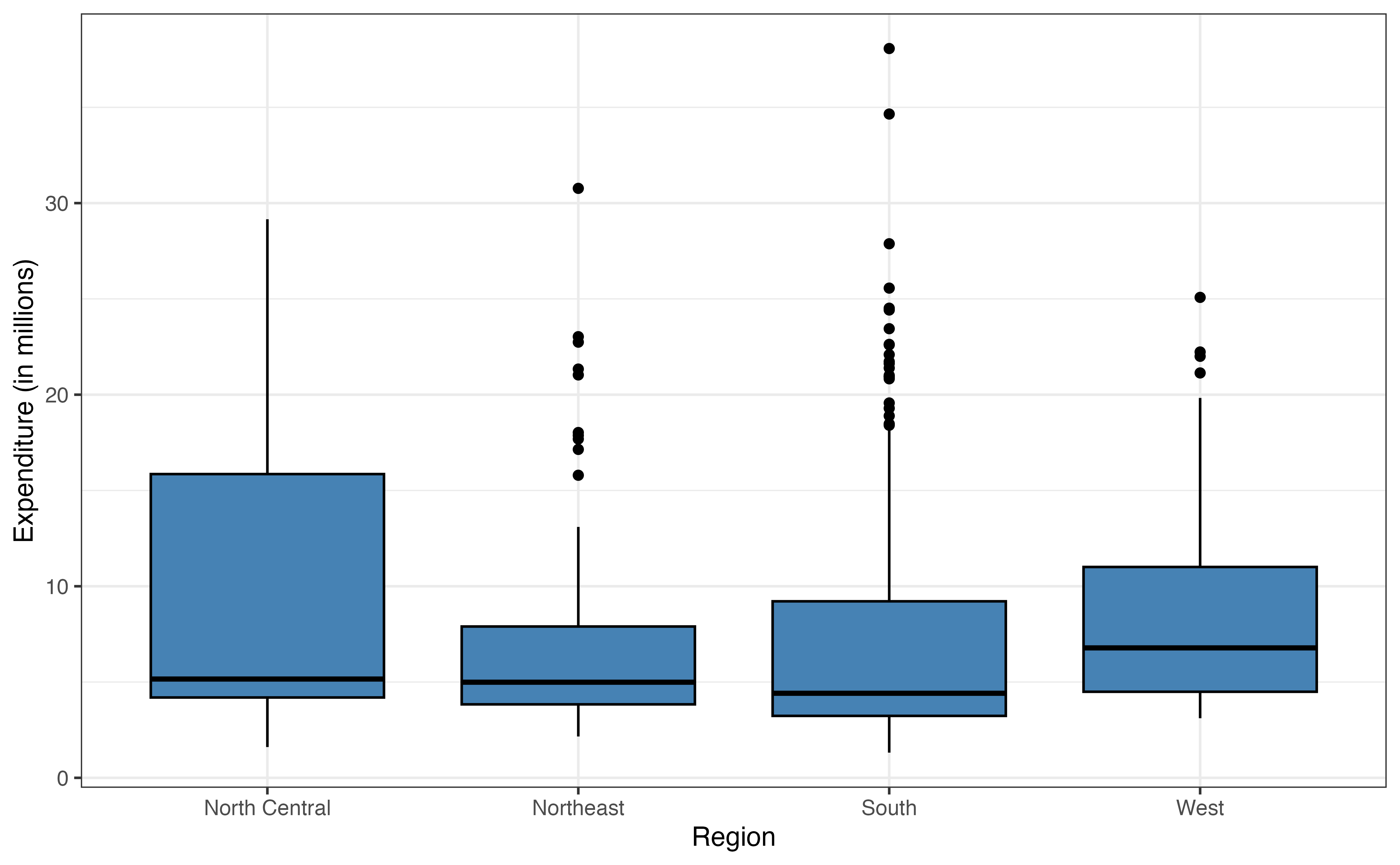
expenditure_m versus region
expenditure_m versus type
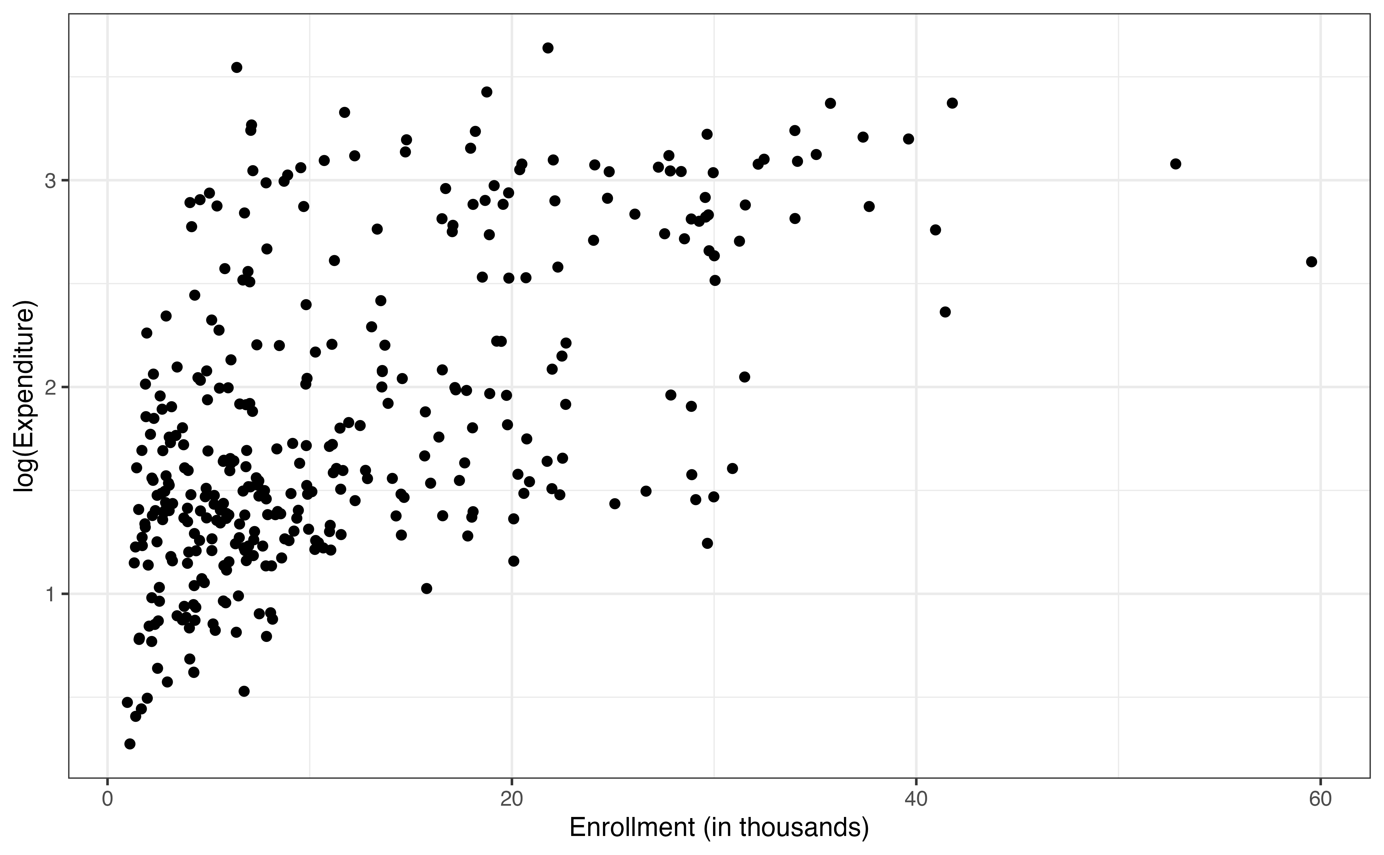
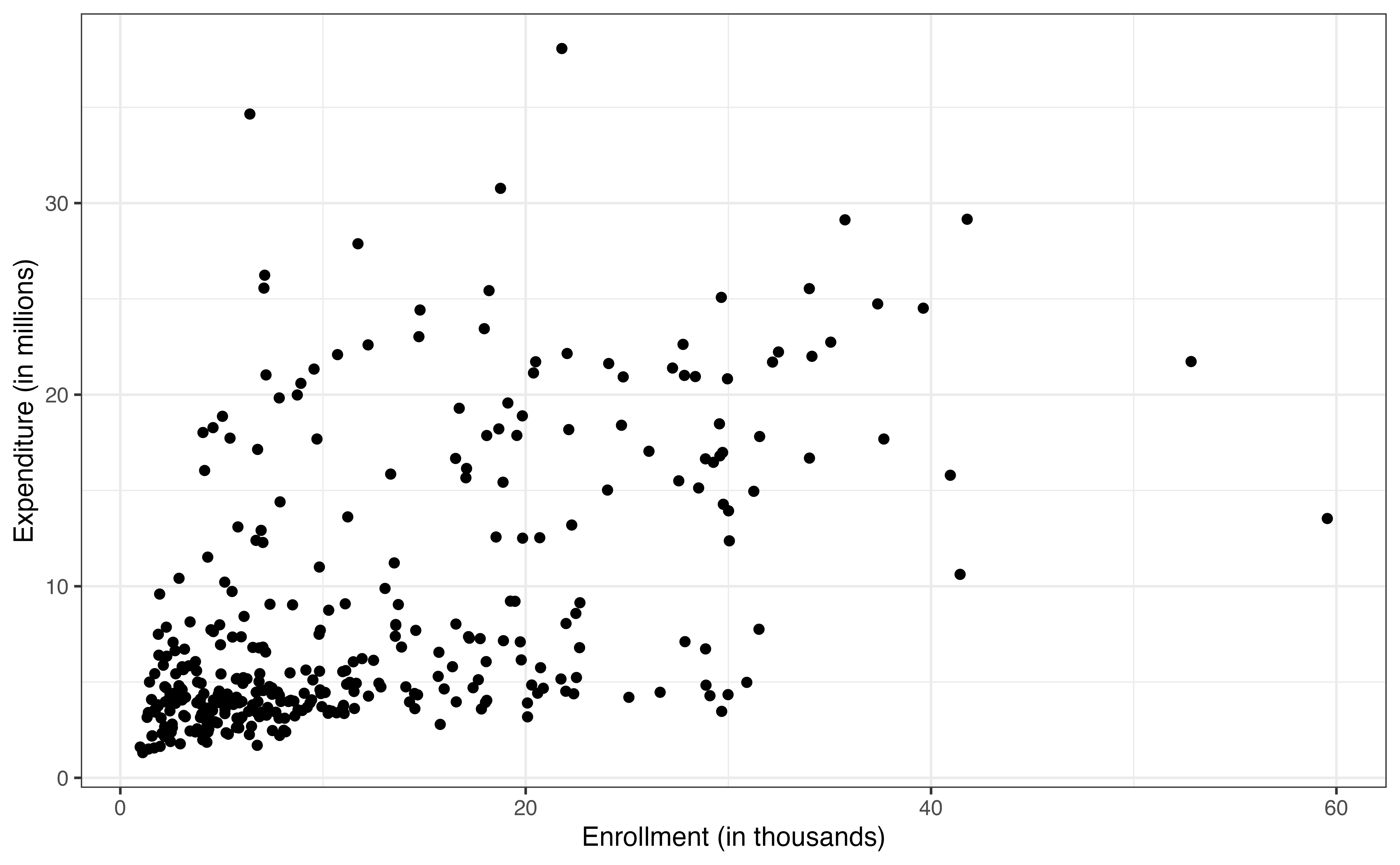
From the bivariate exploratory data analysis in Figure 9.3 (a), there appears to be a strong positive relationship between the enrollment and expenditure. This aligns with what we might expect; colleges with more students are likely to spend more on basketball programs. We note that this trend does seem to level off for colleges with very high enrollment, because their expenditure is lower than what we would expect if expenditure increased as a constant rate for values of enrollment (called monotonically increasing).
The plot also shows two other interesting features of the relationship. The first is that the variability in the expenditure increases as enrollment increases. Thus, there is more variability in how much colleges with larger enrollments spend on basketball programs compared to colleges with small enrollments. We will keep this issue of the changing variability in mind as we fit a model and evaluate the model conditions. The second observation is the appearance of a “V” shape in the trend, indicating two different trajectories. This could be an indication of a potential interaction, so let’s look at multivariate plots to explore a potential interaction between enrollment and type and one between enrollment and region.
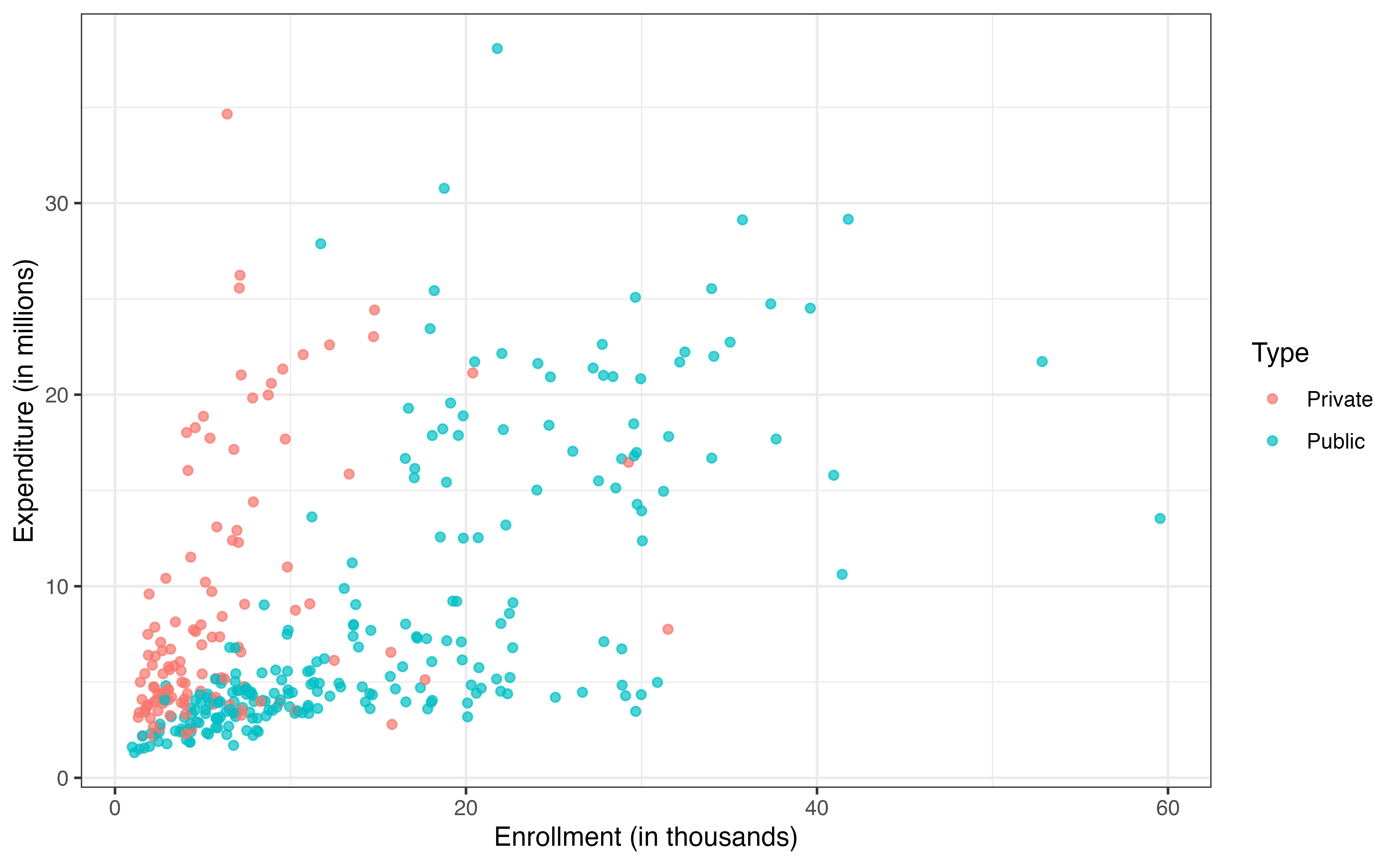
expenditure_m versus enrollment_th by type
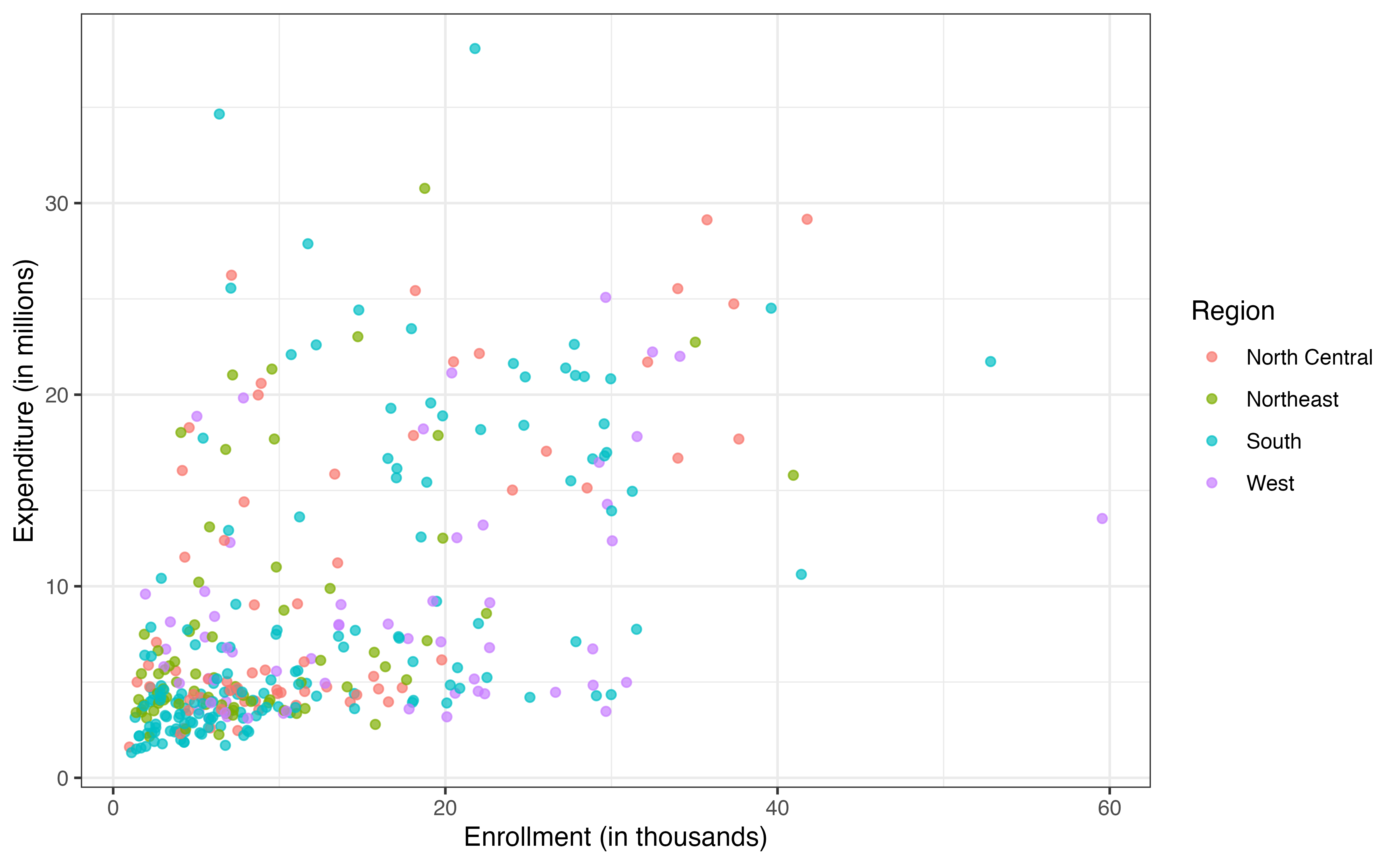
expenditure_m versus enrollment_th by region
Based on the plots in Figure 9.4, do there appear to be any potential interaction effects? Explain.2
We include the interaction between type and enrollment_th in the first modeling attempt, shown in Table 9.2. The plot of the residuals versus fitted values along with the distribution of the residuals are in Figure 9.5.
| term | estimate | std.error | statistic | p.value | conf.low | conf.high |
|---|---|---|---|---|---|---|
| (Intercept) | 7.247 | 1.021 | 7.100 | 0.000 | 5.239 | 9.254 |
| enrollment_th | 0.557 | 0.102 | 5.476 | 0.000 | 0.357 | 0.756 |
| regionNortheast | -3.044 | 0.985 | -3.090 | 0.002 | -4.981 | -1.106 |
| regionSouth | -1.146 | 0.786 | -1.458 | 0.146 | -2.692 | 0.400 |
| regionWest | -3.009 | 0.973 | -3.093 | 0.002 | -4.922 | -1.096 |
| typePublic | -5.049 | 1.042 | -4.845 | 0.000 | -7.099 | -3.000 |
| enrollment_th:typePublic | -0.060 | 0.107 | -0.566 | 0.572 | -0.271 | 0.150 |

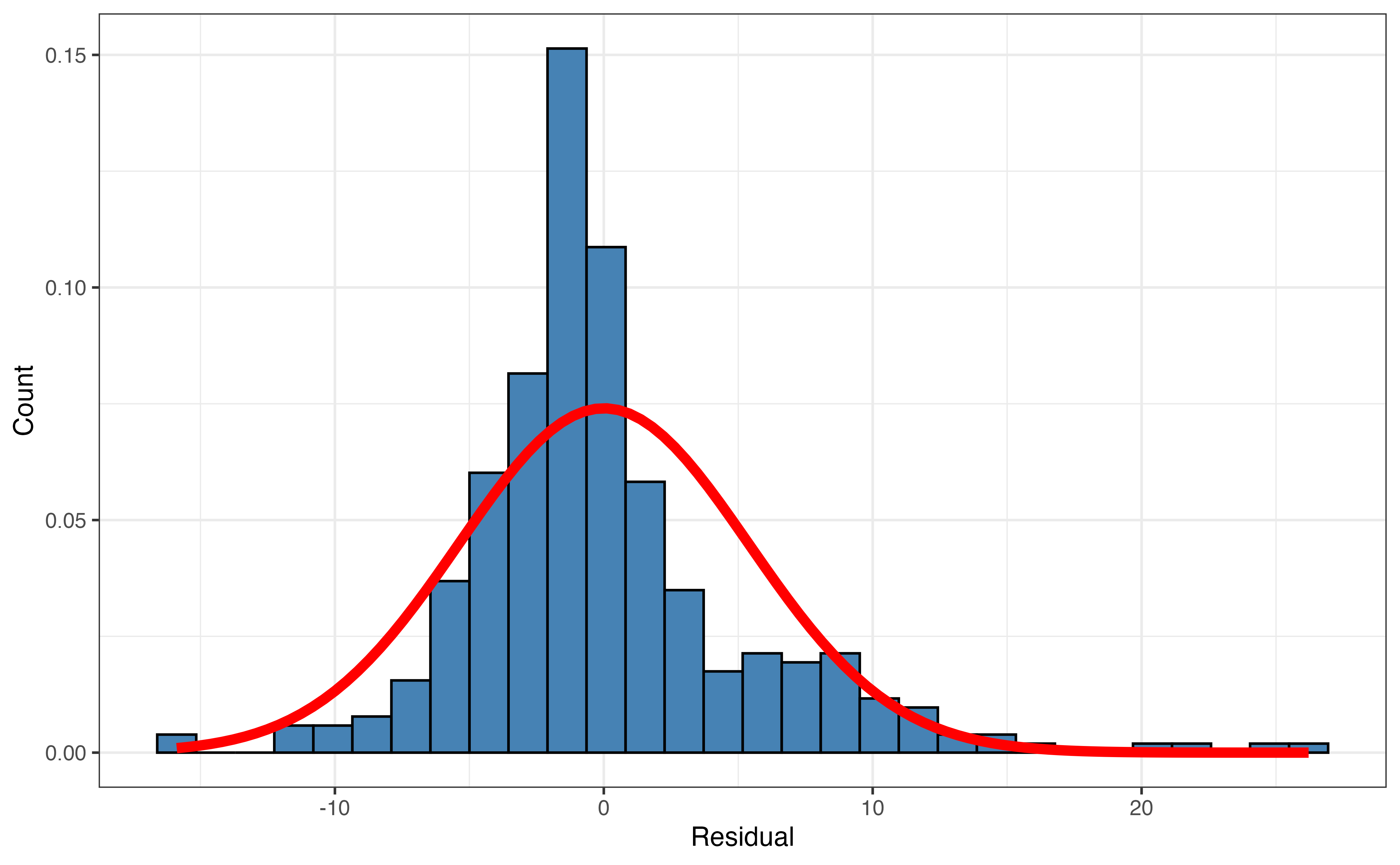
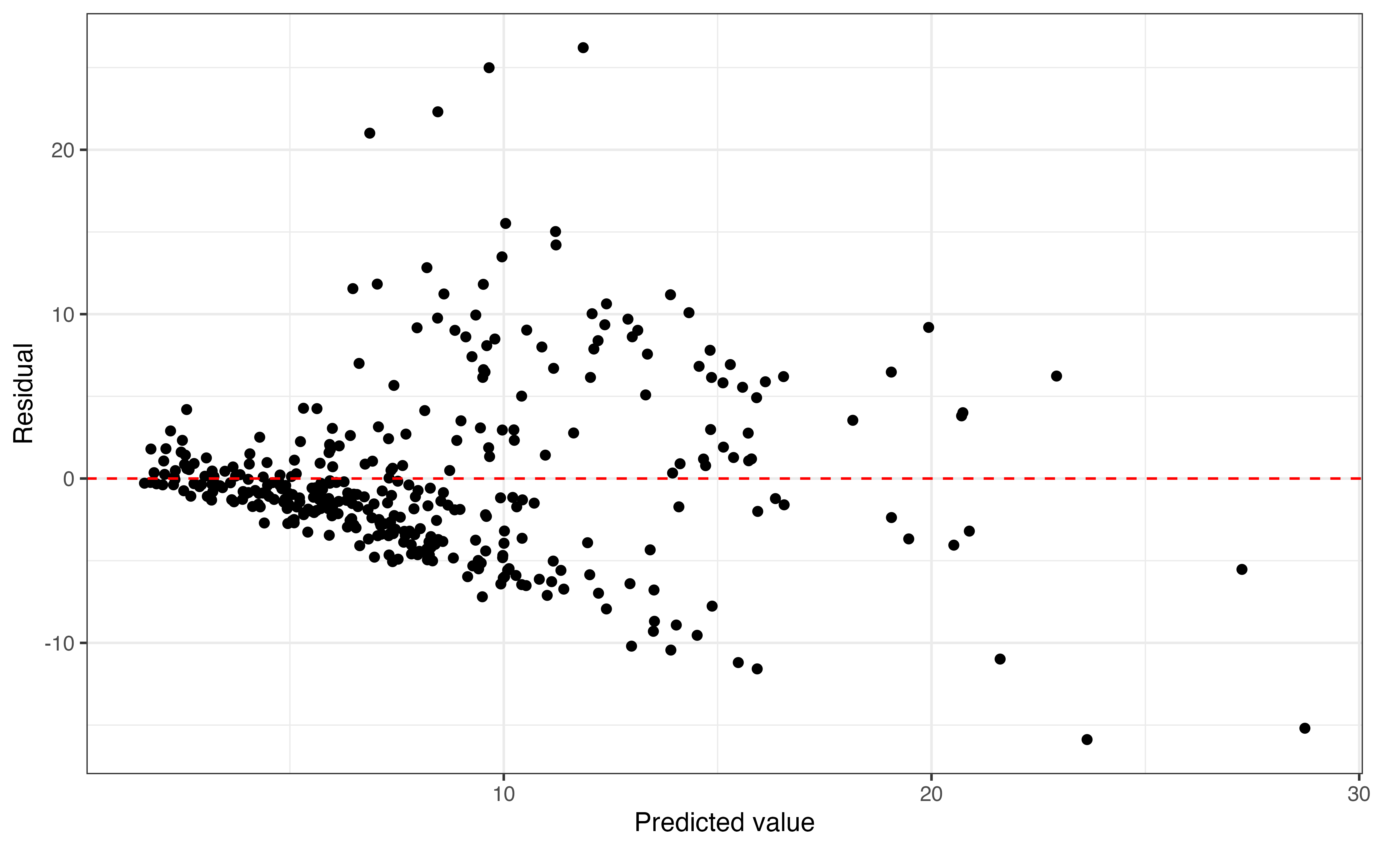
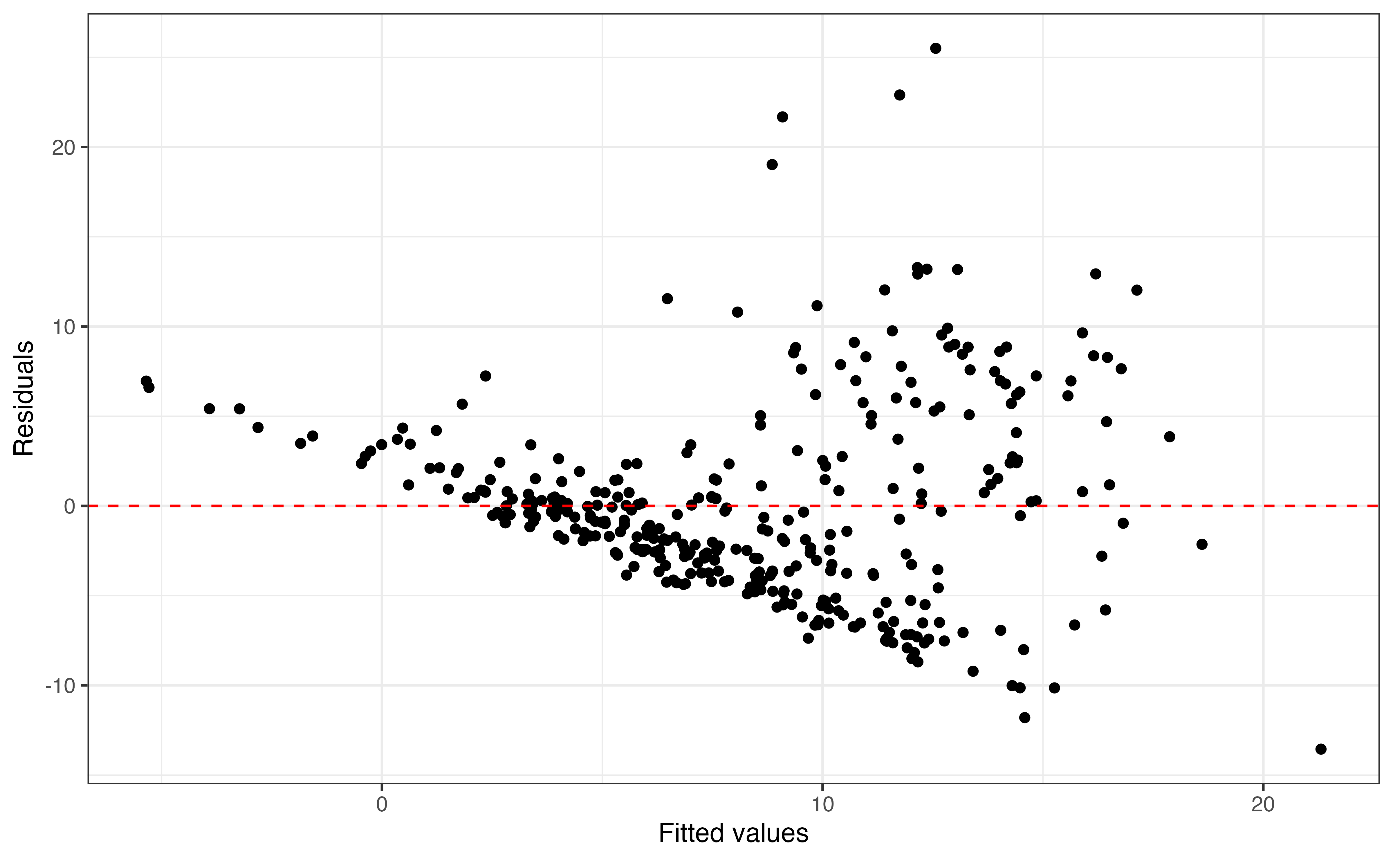
There is a “fan” shape in Figure 9.5, so the equal variance condition is not met. Because the equal variance condition is not met, the results of theory-based inference output in Table 9.2 cannot reliably be used to draw conclusions about the relationships between the response and predictor variables. For example, the inferential results suggest the interaction between enrollment and institution type is not useful in this model, despite what we observed in Figure 9.4. Before making a final conclusion about the interaction term ad any other term in the model, let’s first address the issue with the equal variance condition.
Here is a summary of some of the points of interest we’ve observed thus far in the exploratory data analysis and initial modeling attempt.
The relationship between enrollment_th and expenditure_m seems to “level off” for high-enrollment colleges, thus the relationship may be non-linear.
There is a fan shape in the plot of the residuals versus predicted values, indicating a violation of the equal variance condition.
The exploratory data analysis suggests there is a potential interaction between enrollment_th and type.
Note that items (1) and (2) are about the model fit and item (3) is about a conclusion drawn from the model. Thus we need to address items (1) and (2) before digging further into item (3). To do so, we will examine three additional models that differ based on transformations on the response variable expenditure_m and/or enrollment_th, the quantitative predictor variable. Transformations only apply to quantitative variables, so type and region will remain unchanged in the subsequent models throughout the chapter.
Throughout the chapter, we will interpret the coefficients and evaluate the model conditions for each of the new candidate models. We’ll then use model performance statistics along with the conditions to select the model that best fits the data. The candidate models are the following:

expenditure_m and enrollment_th for four candidate models
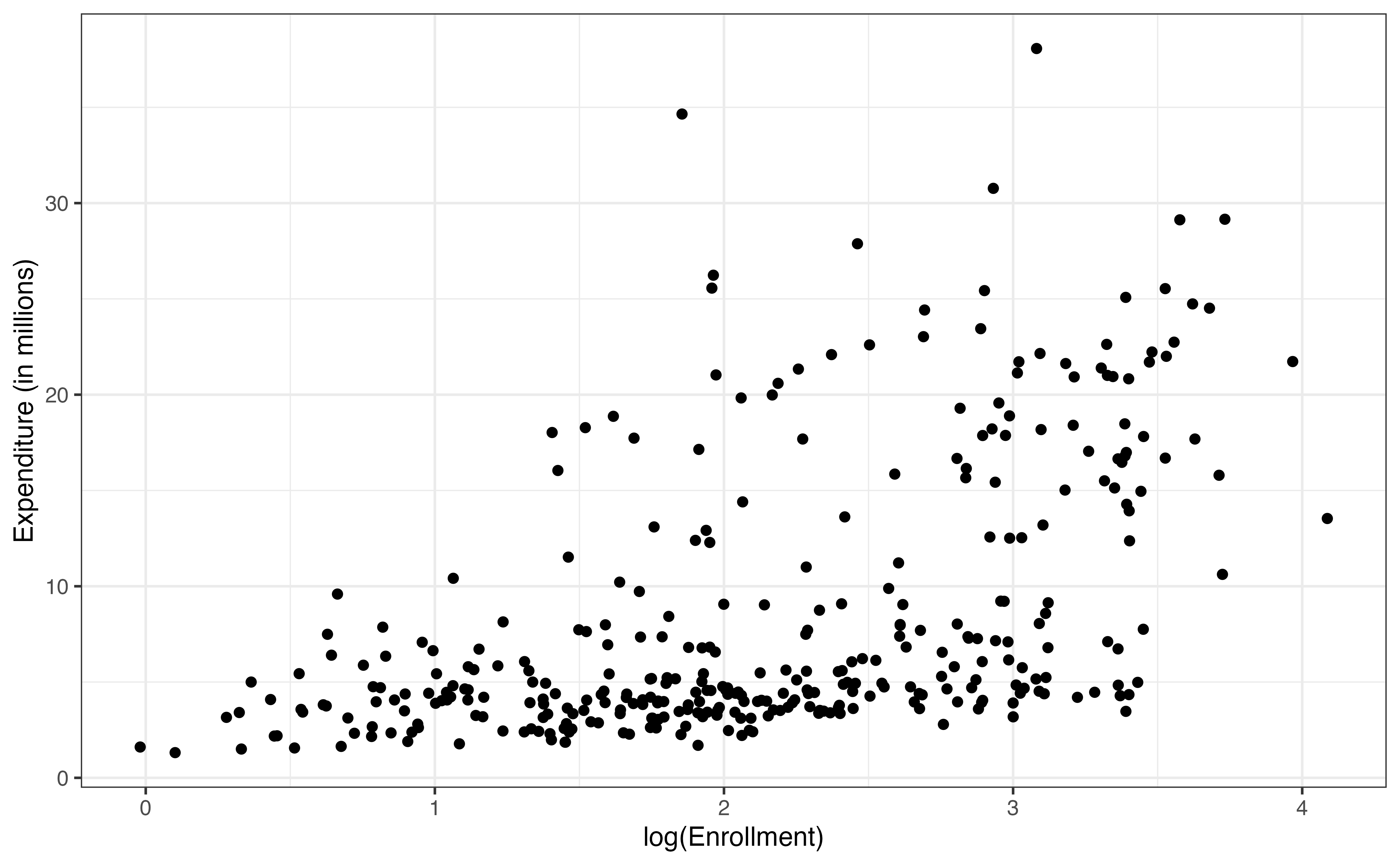
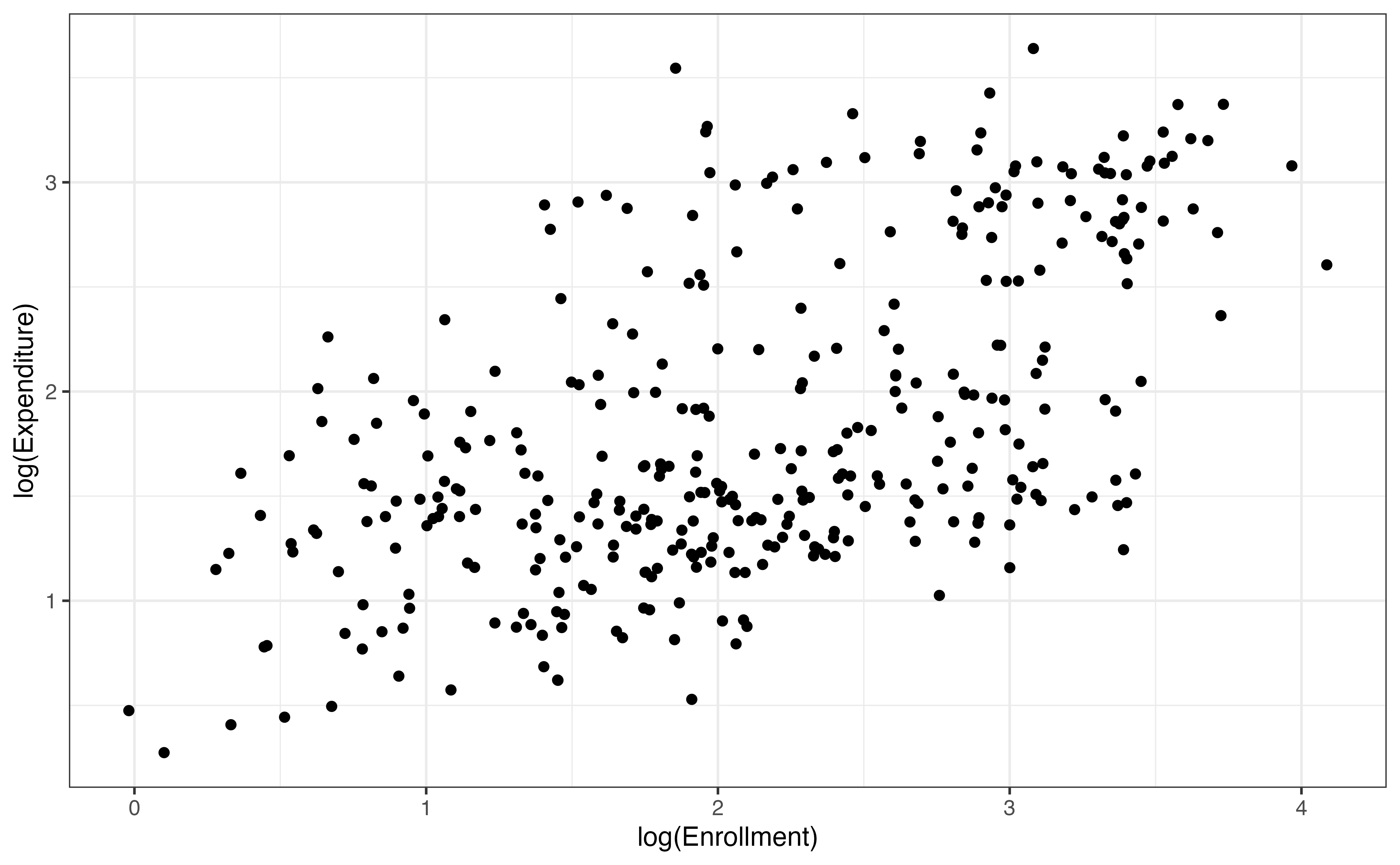
Which relationship visualized in Figure 9.6 would be best summarized by a linear regression model?3
The plots in Figure 9.6 can help provide intuition on what to expect as we do the analysis. In this chapter, we will look at the transformations presented in Plots B - D in the order they are plotted. In practice, however, you can use insights from the exploratory data analysis to start with the model that appears to be the best fit for the data. We do not draw definitive conclusions from the exploratory data analysis, so we will use inference, model conditions, and model fit statistics to select the best fit model. For now, we will just discuss these transformations in terms of a main effects model. In Section 9.5, we add the interaction term to our selected model.
The plot of residuals versus predicted variables in Figure 9.5 shows a clear violation in the equal variance condition based on the fan-shaped pattern of the residuals when moving from left to right. Recall from Section 6.3 that it is necessary to satisfy the equal variance condition when doing theory-based inference (the inference results produced by output), because it relies on a single estimate of \(\hat{\sigma}_{\epsilon}\), the regression standard error (variability about the regression line). We can easily see in Figure 9.5 that a single value would not be representative of the vertical spread of the residuals for all predicted values. Thus, the inferential results in Table 9.2 should be interpreted with caution.
One solution to this is to use the simulation-based inference methods introduced in Section 8.3, because the sampling distribution and null distribution for an estimated coefficient \(\hat{\beta}_j\) are constructed relying only on the data, rather than any underlying assumptions about the distribution of \(\hat{\beta}_j\). Another approach is to use a transformation on the response variable to reduce the impacts of the different vertical spreads in the response variable. Such transformations are called variance-stabilizing transformations.
Some commonly used variance-stabilizing transformations are the square-root transformation, \(\sqrt{y}\) , and the reciprocal transformation, \(1/y\) . In fact, the square root and reciprocal transformations are just two examples from the class of transformations called the Box-Cox transformations (Box and Cox 1964). These transformations are designed to handle a non-normal response variable of any shape. While Box-Cox transformations, such as \(\sqrt{y}\) and \(1/y\), can be the optional choice for stabilizing variance and making the distribution of the response variable more normal (recall the normality condition), it is often difficult to interpret the coefficients for models with such transformed response variables in a way that an be easily understood by readers. Therefore, we will not focus on Box-Cox transformations in this text, because one of our primary objectives is to produce models that are easily interpretable.
Let’s consider another transformation for the response variable that can help address the violations in the equal variance condition while also being easily interpreted by the reader. We can apply a natural log transformation on the response variable, \(\log(y)\) (also written as \(\ln(y)\)), such that \(\log(y)\) has the linear relationship with the predictor variables. Equation 9.1 shows the statistical model when applying such transformation to the response variable.
\[ \log(y_i) = \beta_0 + \beta_1x_{i1} + \beta_2x_{i2}+ \dots + \beta_px_{ip} + \epsilon_i \hspace{8mm} \epsilon_i \sim N(0, \sigma^2_{\epsilon}) \tag{9.1}\]
log = ln
In statistics, the term “log” refers to the natural log (typically denoted \(\ln\) in mathematics).
As shown in Equation 9.1, the log transformation is applied to the individual values of \(Y\), and the transformed values are used in the model. Therefore, when we use a log (or any) transformation on the response variable, we assume the assumptions from Section 5.3 apply to the relationship between the predictors and the transformed values of \(Y\). Using Equation 9.1, this means we make assumptions about the relationship between the predictors and \(\log(y_i)\). The full analysis, including evaluating conditions and diagnostics, conducting inference, and computing predictions are done in terms of \(\log(y)\). Interpretations, however, are in terms of the original variable \(y\). Although we can write interpretations in terms of \(\log(y)\) (we’ll see an example of this shortly), it is not as intuitive for readers to understand interpretations on a log-scale as on the natural scale.
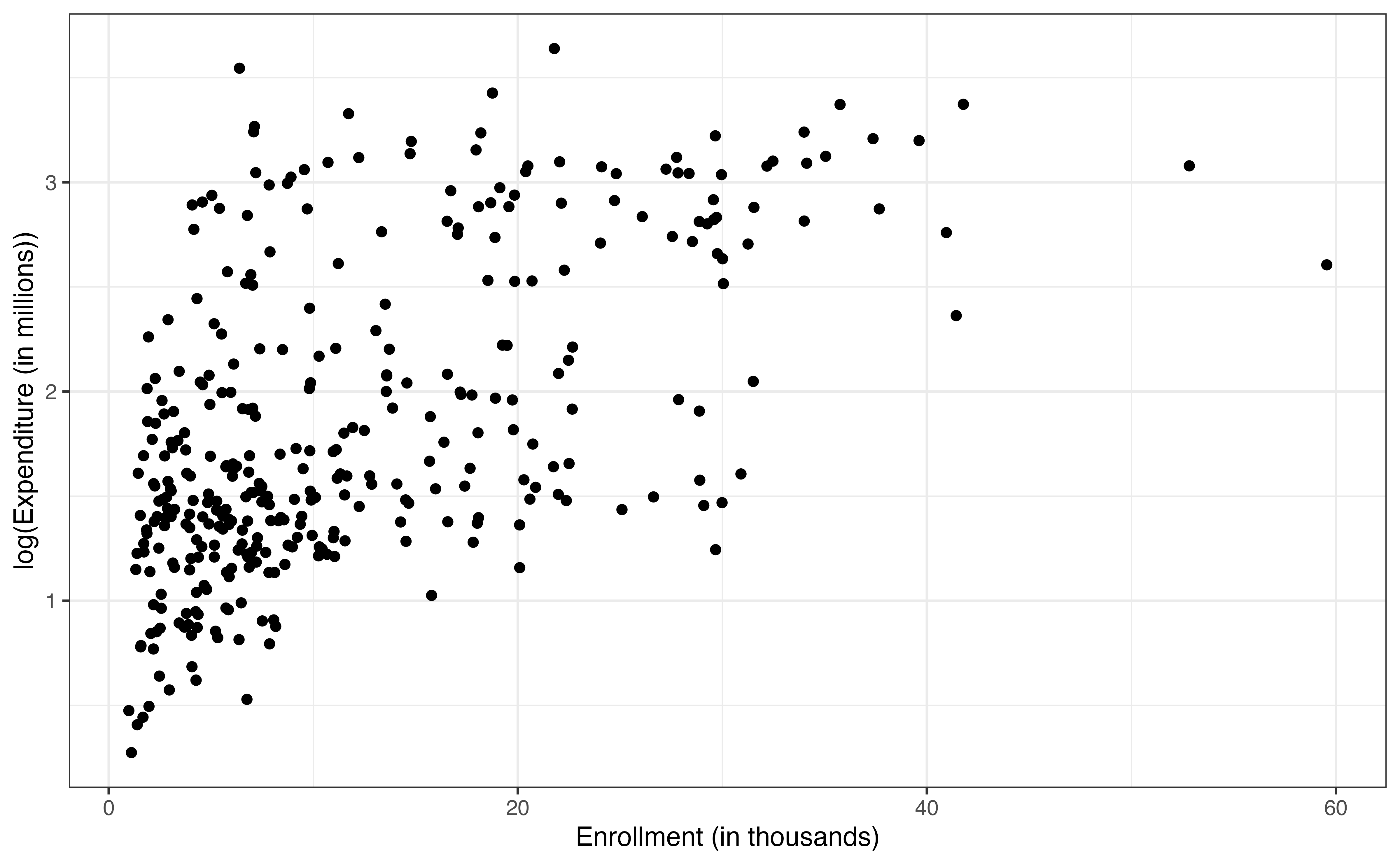
Let’s begin by looking at the distribution of log(expenditure_m), its relationship with enrollment_th, and how these compare to the exploratory data analysis in Section 9.1.
expenditure_m
expenditure_m
expenditure_m versus enrollmenth_th
expenditure_m versus enrollment_th
expenditure_m
Now we fit the main effects model using log(expenditure_m), the log-transformed expenditure, as the response variable. The output for the new is in Table 9.3 and the equation is in Equation 9.2.
| term | estimate | std.error | statistic | p.value | conf.low | conf.high |
|---|---|---|---|---|---|---|
| (Intercept) | 1.783 | 0.084 | 21.21 | 0.000 | 1.617 | 1.948 |
| enrollment_th | 0.056 | 0.003 | 17.14 | 0.000 | 0.050 | 0.062 |
| regionNortheast | -0.311 | 0.098 | -3.19 | 0.002 | -0.503 | -0.119 |
| regionSouth | -0.176 | 0.078 | -2.26 | 0.025 | -0.329 | -0.023 |
| regionWest | -0.218 | 0.096 | -2.26 | 0.024 | -0.408 | -0.028 |
| typePublic | -0.672 | 0.074 | -9.11 | 0.000 | -0.817 | -0.527 |
\[ \begin{aligned} \widehat{\log(\text{expenditure\_m})} = & 1.783 + 0.056 \times \text{enrollment\_th}\\ &- 0.311 \times \text{Northeast} - 0.176 \times \text{South} \\ & - 0.218 \times \text{West} - 0.672 \times \text{Public} \end{aligned} \tag{9.2}\]
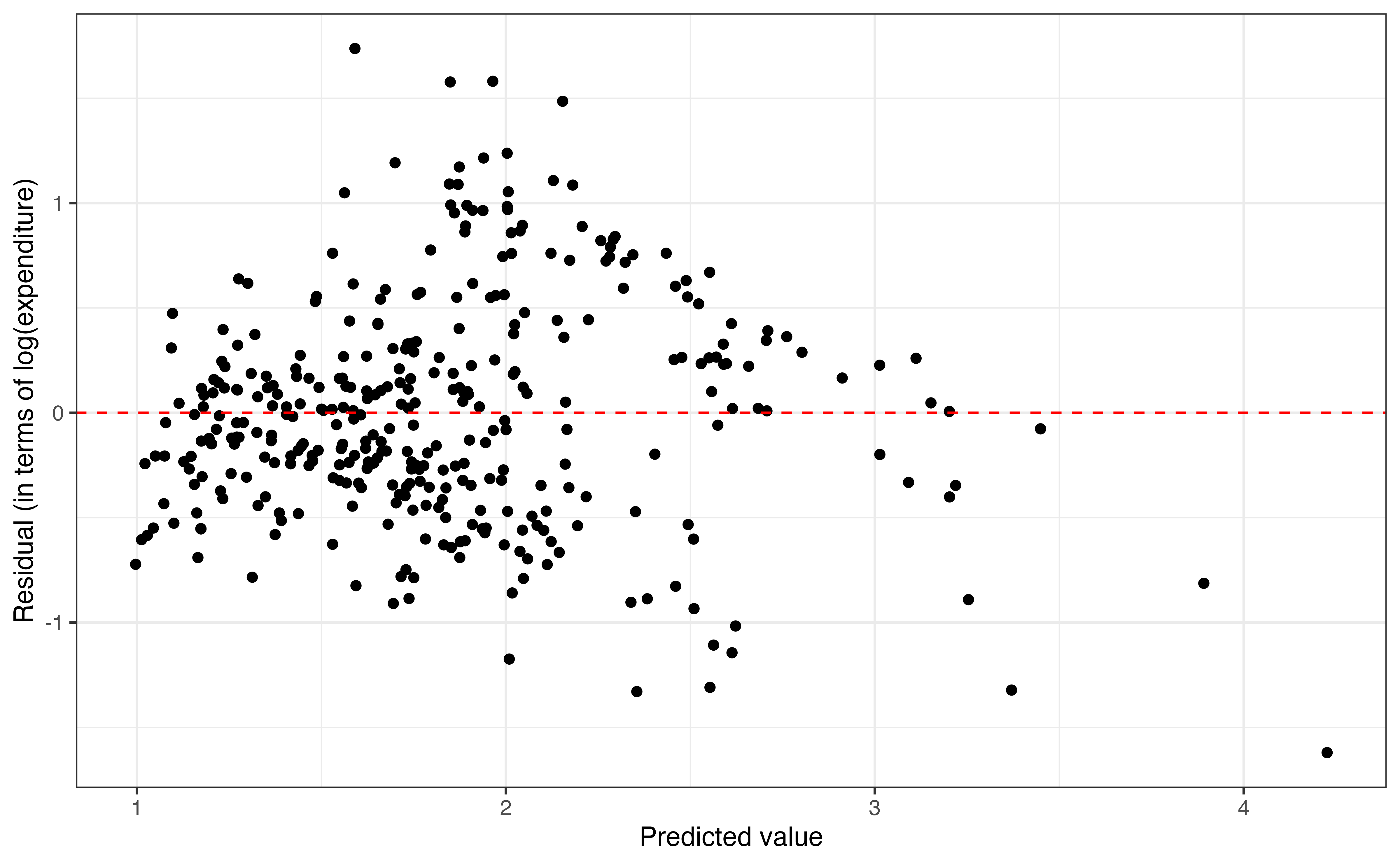
Before using the model, we analyze the residuals versus predicted values to evaluate whether the concerns with equal variance have been addressed by the transformation. Figure 9.8 shows the original plot of the residuals versus predicted values and the plot for the model using the log-transformed response variable.
expenditure_m
expenditure_m
Comparing the plots in Figure 9.8, the first observation is that the \(y\)-axis differs on the plots. This is the because the residuals are on the same scale and use the same units as the response variable. The residuals in Figure 9.8 (a) are in terms of the original variable expenditure_m, and the residuals in Figure 9.8 (b) are in terms of log(expenditure_m). The same is true for the predicted values on the \(x\)-axis. The second observation is that the vertical spread of the residuals is much more equal Figure 9.8 (b) with the log-transformed response variable. Given this, it appears applying a log transformation on the response variable has addressed some of the problems with the equal variance condition.
We can consider other transformations to improve the model fit even more; we’ll discuss those as the chapter continues. For now, let’s interpret the coefficients for the model in Table 9.3. The approach for interpreting the model coefficients in terms of the log-transformed response variable is the same as the one introduced in Section 9.2 for other multiple linear regression models. Below are the interpretations for enrollment_th and regionNortheast in terms of log(expenditure).
For each additional 1000 students at an NCAA Division I college, the total log(expenditure) on basketball programs is expected to increase by 0.056 log(millions of dollars), on average, holding region and type constant.
The total log(expenditure) on basketball programs for NCAA Division I colleges is expected to be 0.311 log(millions of dollars) less, on average, for colleges in the Northeast region compared to those in the North Central region, holding enrollment and type constant.
Though these interpretations are technically correct, it is difficult to fully comprehend what a change in log(millions of dollars) to the log(expenditure) really means. Therefore, we need to get back to the original variable (expenditure_m) and back to the original units (millions of dollars) to write an interpretation that is more intuitive.
\(e^{\log(a)} = a\)
\(e^{a+b} = e^ae^b\)
Given Equation 9.1 with a log-transformed response variable, the predicted values in terms of the original response variable is
\[ \begin{aligned} \hat{y}_i &= e^{\hat{\beta}_0 + \hat{\beta}_1x_{i1} + \hat{\beta}_2x_{i2}+ \dots + \hat{\beta}_px_{ip}} \\[10pt] & = e^{\hat{\beta}_0}e^{\hat{\beta}_1x_{i1}}e^{\hat{\beta}_2x_{i2}} \dots e^{\hat{\beta}_px_{ip}} \end{aligned} \tag{9.3}\]
From Equation 9.3, the interpretations in terms of the original response variable are about a multiplicative change in the response when the predictor variable changes. Specifically, when \(X_j\) increases by one unit, \(Y\) is expected to multiply by a factor of \(e^{\hat{\beta}_j}\). The mathematical details for Equation 9.3 and the interpretations are in Section A.9.1.
Now let’s use Equation 9.3 to interpret the coefficients of enrollment_th and regionNortheast in terms of expenditure_m.
For each additional 1000 students at an NCAA Division I college, the total log(expenditure) on basketball programs is expected to multiply by a factor of 1.058 (\(e^{0.056}\)), holding region and type constant.
The total expenditure on basketball programs for NCAA Division I colleges in the Northeast region is expected to be 0.733 (\(e^{-0.311}\)) times the expenditure at colleges in the North Central region, holding enrollment and type constant.
The intercept, the expected response when all predictors are equal to 0, is \(e^{\hat{\beta}_0}\). Thus, the interpretation of the intercept for Table 9.3 in terms of the original response variable is
The total expenditure on basketball programs for private NCAA Division I colleges in the North Central region with no students enrolled is expected to be 5.948 \((e^{1.783})\) million dollars.
Transformations on the response variable are often done to address violations in the equal variance condition, as shown in the previous section. In this section, we introduce transformations on one or more quantitative predictor variables that are used to model non-linear relationships with the response variable.
In the exploratory data analysis in Section 9.1.1, we observed that the relationship between expenditure_m and enrollment_th flattened as enrollment_th increased. For Colleges with larger enrollments generally have a smaller increase in expenditures on basketball programs for each additional 1000 students compared to the increase in expenditures for colleges with smaller enrollments. We account for this decreasing effect by applying a log transformation on the predictor variable. Here we will transform a single predictor but we can apply a log transformation to multiple quantitative predictors in a model.
The general form of the linear regression model with a log-transformed predictor variable \(x_j\) is shown in Equation 9.4 .
\[ y_i = \beta_0 + \beta_1x_{i1} + \dots + \beta_j\log(x_{ij}) + \dots + \beta_px_{ip} + \epsilon_i \hspace{5mm} \epsilon_i \sim N(0, \sigma^2_{\epsilon}) \tag{9.4}\]
Equation 9.5 shows the form of the model for NCAA Division I basketball expenditure using log-transformed values of enrollment.
\[ \begin{aligned} \text{expenditure\_m}_i = \beta_0 &+ \beta_1 \log(\text{enrollment\_th}_i) + \beta_2\text{Northeast}_i + \beta_3\text{South}_i \\ &+ \beta_4\text{West}_i + \beta_5\text{Public}_i + \epsilon_i \hspace{5mm} \epsilon_i \sim N(0, \sigma^2_{\epsilon}) \end{aligned} \tag{9.5}\]
At this point, we are using the original response variable, expenditure_m, so we can focus on understanding the log-transformed predictor variable. In the next section, we will look at the scenario in which both the response variable and one or more predictor variables is transformed. The output of the model with log-transformed enrollment is in Table 9.4.
enrollment_th
| term | estimate | std.error | statistic | p.value |
|---|---|---|---|---|
| (Intercept) | 1.297 | 1.026 | 1.265 | 0.207 |
| log(enrollment_th) | 5.992 | 0.400 | 14.994 | 0.000 |
| regionNortheast | -3.242 | 0.991 | -3.271 | 0.001 |
| regionSouth | -0.662 | 0.793 | -0.835 | 0.404 |
| regionWest | -2.919 | 0.978 | -2.985 | 0.003 |
| typePublic | -6.531 | 0.783 | -8.337 | 0.000 |
Let’s start by interpreting the intercept for this model. Because we have used the log-transformed value of enrollment in the model, the intercept represents the subgroup of NCAA Division 1 colleges such that log(enrollment_th) and all the other predictors are equal to 0. Based on the rules of logarithms, log(enrollment_th) is equal to 0 when enrollment_th is equal to 1, corresponding to an institution with 1000 students enrolled. The interpretation of the intercept for this model is the following:
The expenditure on basketball programs for private NCAA Division 1 colleges in the North Central region with 1000 students enrolled (
log(enrollment_th) = 0) is expected to be 1.297 million dollars.
Now let’s look at the interpretation of the predictor variable enrollment_th. Using the coefficient interpretations introduced in Section 7.4.1, the interpretation is the following:
When the log-transformed enrollment increases by 1, the expenditure on basketball programs at NCAA Division 1 colleges is expected to increase by 5.992 million dollars, holding type and region constant.
Though this interpretation is technically accurate, it is difficult to comprehend what an increase in the log-transformed enrollment actually means. Therefore, rather than interpreting the coefficient in terms of the log-transformed enrollment, we interpret enrollment in terms of its original units of 1000 students.
Because `enrollment_th` is on the logarithmic scale in the model, it is most straightforward to interpret the change in expenditure when enrollment is multiplied by a constant \(C\). In general terms, given a model of the form in Equation 9.4, the interpretation of predictor \(X_j\) is below. The mathematical details for this interpretation are in Section A.9.2.
When \(X_j\) is multiplied by a constant \(C\), \(Y\) is expected to change (increase or decrease) by \(\beta_j \log(C)\) units, holding all else constant.
\(\log(ab) = \log(a) + \log(b)\)
Applying this to Equation 9.4,
\(\beta_j\log(CX_j) = \beta_j[\log(C) + \log(X_j)] = \beta_j\log(C) + \beta_j \log(X_j)\)
Now let’s interpret the effect of enrollment_th in terms of the expected change in expenditure_m when enrollment_th doubles (\(C = 2\)).
When the enrollment doubles (is multiplied by 2), the expenditure on basketball programs at NCAA Division 1 institutions is expected to increase by 4.153 (5.992 \(\times\) log(2)) million dollar, on average, holding type and region constant.
When writing these interpretations, the constant \(C\) can take any value between \(-\infty\) and \(\infty\). When choosing \(C\), however, we need to be mindful about potential extrapolation and writing interpretations for values far outside the range of the data. Use values of \(C\) between 1 and 2 to reduce potential extrapolation. Values in this range provide straightforward interpretations about the expected change when there is some percentage increase in the predictor (for example, \(C = 1.1\) equals a 10% increase in the value of the predictor). Note, however, that there is a risk of extrapolating for observations with values at or near the maximum value of the predictor. For example, there is a college in the data with enrollment around 59,000. We should be cautious when using the model to interpret the expected change when enrollment doubles for this institution. This would equal an enrollment of over 118,000 students, which is far outside the range of the data. We cannot safely assume the relationship between enrollment_th and expenditure_m observed in Table 9.4 is the same for colleges with such high enrollment (or that such colleges even exist!).
Write the interpretation of the expected change in expenditure on basketball programs when enrollment increases by 50% \((C = 1.5)\).6
enrollment_th
The plot of the residuals versus fitted values for the model Table 9.4 is shown in Figure 9.9. This plot has a fan shape similar to the one observed in Figure 9.5. Therefore, even though the log transformation on enrollment_th accounted for its non-linear relationship with expenditure_m, it did not address the violation in the equal variance condition like the log transformation on the response variable in Section 9.2. In the next section, we introduce a model that includes both a log-transformed response variable and log-transformed predictor.
Models with transformations on both the response variable and one or more quantitative predictor variables can both address violations in the equal variance condition and capture non-linear relationships. Given what we have observed in the exploratory data analysis in Section 9.1.1 and the residual plots in Figure 9.5, Figure 9.8 , and Figure 9.9, we will now fit a model using both log(expenditure_m) and log(enrollment_th).
Equation 9.6 is the general form of the model with a log-transformed response variable and a log-transformed predictor variable \(x_j\) is shown in
\[ \log(y_i) = \beta_0 + \beta_1x_{i1} + \dots + \beta_j\log(x_{ij}) + \dots + \beta_px_{ip} + \epsilon_i \hspace{5mm} \epsilon_i \sim N(0, \sigma^2_{\epsilon}) \tag{9.6}\]
Equation 9.7 shows the form of the model for NCAA Division I basketball expenditure, and the output of the estimated model is in Table 9.5.
\[ \begin{aligned} \log(\text{expenditure\_m}_i) = \beta_0 &+ \beta_1 \log(\text{enrollment\_th}_i) + \beta_2\text{Northeast}_i + \beta_3\text{South}_i \\ &+ \beta_4\text{West}_i + \beta_5\text{Public}_i + \epsilon_i \hspace{5mm} \epsilon_i \sim N(0, \sigma^2_{\epsilon}) \end{aligned} \tag{9.7}\]
| term | estimate | std.error | statistic | p.value |
|---|---|---|---|---|
| (Intercept) | 1.025 | 0.097 | 10.58 | 0.000 |
| log(enrollment_th) | 0.707 | 0.038 | 18.75 | 0.000 |
| regionNortheast | -0.337 | 0.094 | -3.60 | 0.000 |
| regionSouth | -0.115 | 0.075 | -1.53 | 0.126 |
| regionWest | -0.221 | 0.092 | -2.39 | 0.017 |
| typePublic | -0.830 | 0.074 | -11.22 | 0.000 |
To interpret the model in Table 9.5 that has both a log-transformed response and predictor variable, we will combine the approach to interpretations from Section 9.2 and Section 9.3.
The intercept is the expected value of log(y) when all the predictors are equal to 0. Because there is a log-transformed predictor \(x_j\) in the model in Equation 9.6, this will be when \(\log(x_j)\) is equal to 0, meaning \(x_j\) is equal to 1. In terms of the model on NCAA Division I basketball expenditures shown in Table 9.5, the intercept 1.025 is interpreted as follows:
The expected log-transformed expenditure on basketball programs at private NCAA Division I colleges in the North Central region with 1000 students enrolled is 1.025.
For readability, we won’t present results in terms of log-transformed expenditure, so we get back to the original response variable expenditure_m.
The expected expenditure on basketball programs at private NCAA Division I colleges in the North Central region with 1000 students enrolled is 2.787 (exp(1.025)) million dollars.
The interpretation for \(\beta_j\), the coefficient for \(\log(X_j)\) in Equation 9.6 is a bit more involved, as it incorporates the multiplicative change in both \(X\) and \(Y\). We’ll start by writing the interpretation in terms of \(\log(Y)\).
When \(X_j\) multiplies by a factor of \(C\), \(\log(Y)\) is expected to change (increase or decrease) by \(\beta_j \log(C)\) , on average, holding all else constant.
\(e^{a\log(b)} = b^a\)
Note that this interpretation is very similar to the interpretation from Section 9.3, when there is a log-transformed predictor variable. The full mathematical details to get back to the original response variable are in Section A.9.3 .The final interpretation in terms of the original response variable when \(X_j\) is multiplied by \(C\) is
When \(X_j\) multiplies by a factor of \(C\), \(Y\) is expected multiply by a factor of \(C^{\beta_j}\) , holding all else constant.
Now let’s use this to interpret enrollment_th for the model in Table 9.5. Below is the interpretation in terms of a 20% increase in enrollment, \(C = 1.2\).
When enrollment at NCAA Division I colleges increases by 20% (multiples by 1.2), the expenditure on basketball programs is expected to multiply by a factor of 1.138 ( \(1.2^{0.707}\)), holding type and region constant.
Write the interpretation for typePublic in Table 9.5 in the context of the data. Write the interpretation in terms of the original variable expenditure_m. 7
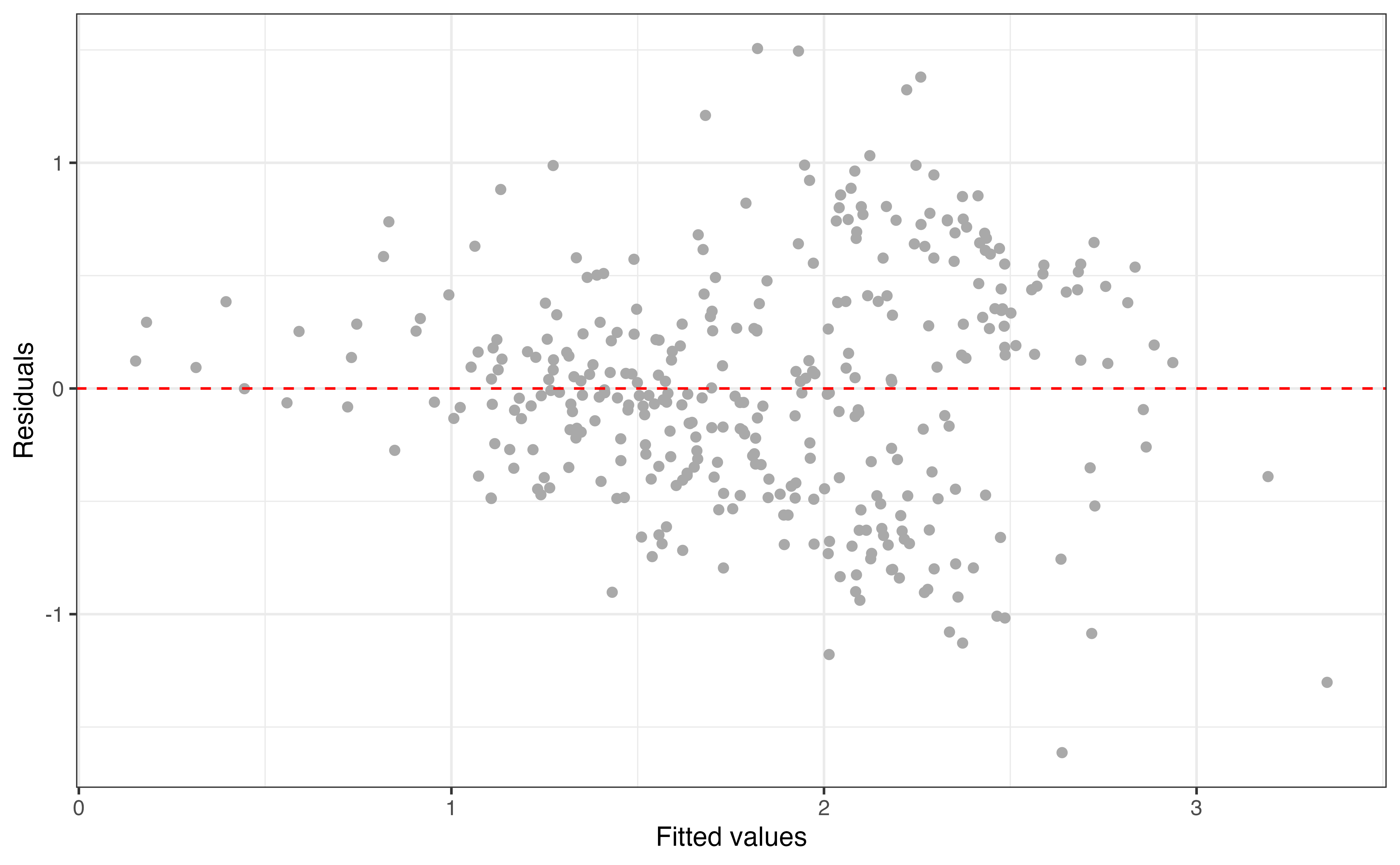
The plot of residuals versus predicted for the model in Table 9.5 is shown in Figure 9.10. This plot shows improvement in the equal variance condition compared to the original residuals plot in Figure 9.5, given the vertical spread of the residuals is more equal around the majority of the data. There is less variability in the residuals for institutions with low predicted expenditure, but there are few institutions with predicted log(expenditure) less than 1.
So far we have looked at four potential models using enrollment_th, type and region to understand variability in expenditure_m. The next step is to select one of these models to use for prediction and inference based on the original analysis objectives. In addition to checking the residual plots and model conditions, we use performance statistics, such as \(R^2\), to help select the model that best fits the data. We discuss model evaluation and selection in-depth in Chapter 10.
| Original | log(y) | log(x) | log(x) & log(y) |
|---|---|---|---|
| 0.409 | 0.473 | 0.4 | 0.516 |
Table 9.6 shows the \(R^2\) values for the four candidate models. Based on the \(R^2\) values and the plots of the residuals versus predicted values, the model that includes both log(expenditure_m) and log(enrollmet_th) is the one that best fits the data.
Now that we have selected the main effects, let’s reconsider the interaction between enrollment_th and type. Figure 9.11 visualizes log(expenditure_m) versus log(enrollment_th) by type to see if there is a potential interaction effect using the transformed variables.
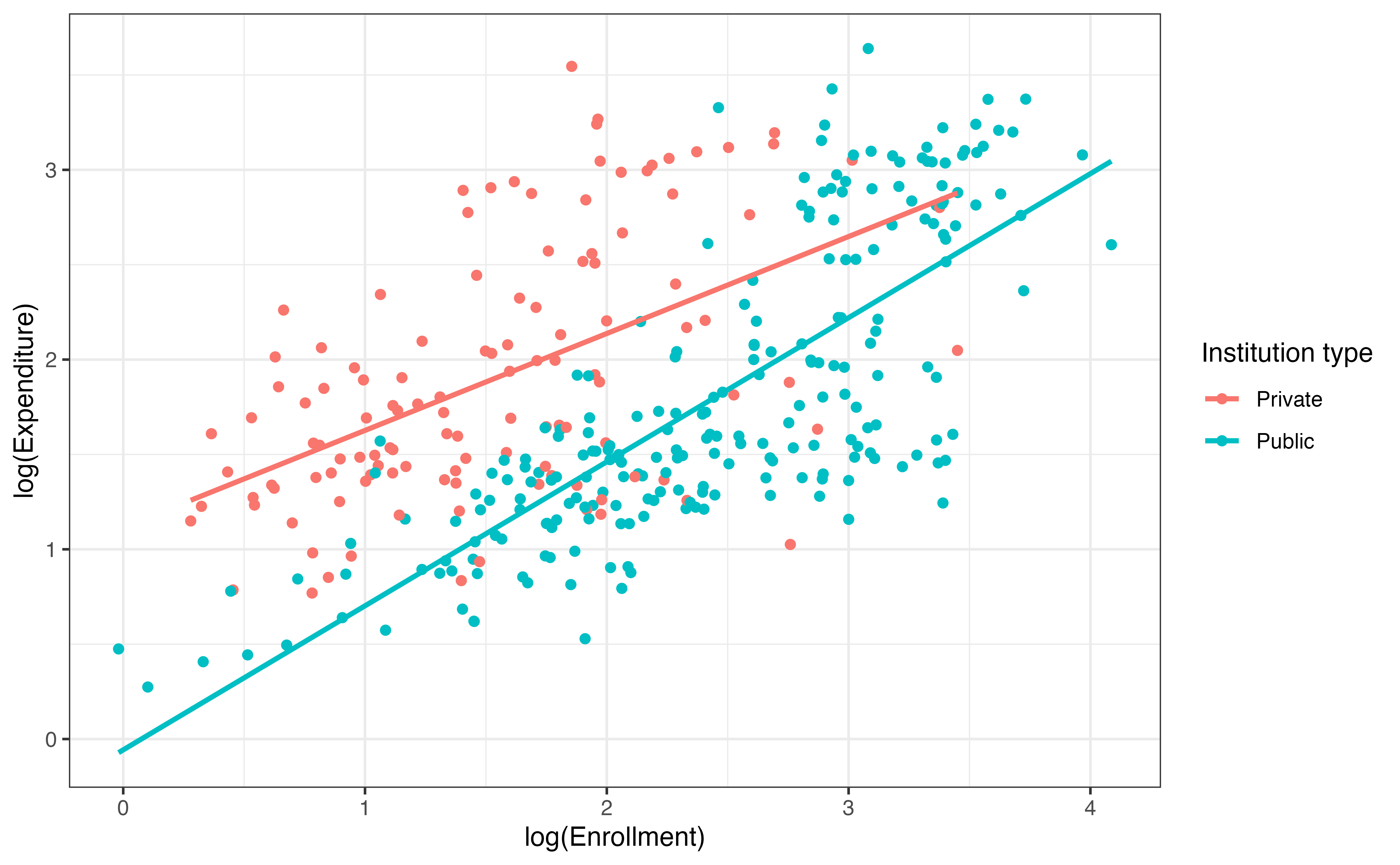
The plot shows that there may be an interaction effect, because the slope of the relationship between log(expenditure_m) and log(enrollment_th) is steeper for public colleges than for private colleges. Given this plot, we include the interaction term to the model selected in Section 9.5. The output is in Table 9.7.
| term | estimate | std.error | statistic | p.value | conf.low | conf.high |
|---|---|---|---|---|---|---|
| (Intercept) | 1.308 | 0.131 | 9.96 | 0.000 | 1.050 | 1.566 |
| log(enrollment_th) | 0.524 | 0.069 | 7.58 | 0.000 | 0.388 | 0.660 |
| regionNortheast | -0.339 | 0.092 | -3.67 | 0.000 | -0.521 | -0.158 |
| regionSouth | -0.117 | 0.074 | -1.58 | 0.114 | -0.262 | 0.028 |
| regionWest | -0.232 | 0.091 | -2.54 | 0.011 | -0.411 | -0.053 |
| typePublic | -1.284 | 0.162 | -7.94 | 0.000 | -1.602 | -0.966 |
| log(enrollment_th):typePublic | 0.255 | 0.081 | 3.15 | 0.002 | 0.095 | 0.414 |
The confidence interval for log(enrollment_th):typePublic gives evidence that the interaction is useful to include in the model. Additionally, the \(R^2\) for this model is 0.53, which is higher than the model chosen from Table 9.6. The equation for the model with the interaction term is
\[ \begin{aligned} \widehat{\log(\text{expenditure\_m}_i)} &= 1.308 + 0.524 \times \log(\text{enrollment\_th}_i)\\ &- 0.339 \times \text{Northeast}_i - 0.117 \times \text{South}_i \\ &- 0.232 \times \text{West}_i - 1.284 \times \text{Public}_i \\ & + 0.255 \times \log(\text{enrollment\_th}_i) \times \text{Public}_i \end{aligned} \]
We put together the concepts from Section 7.7 and Section 9.4 to interpret the model coefficients describing the relationship between enrollment_th, type, and expenditure_m on basketball programs. The coefficient of the interaction term \(\hat{\beta}_{interaction} = 0.255\) means that \(\log(\text{expenditure})\) changes (increases or decreases) by an additional \(C \times 0.255\) for public colleges compared to private colleges when enrollment is multiplied by a factor \(C\). This means that the expenditure is expected to multiply by an additional \(C^{0.255}\) for public institutions compared to private ones.
Below are the interpretations of the relationship between enrollment and expenditure for public and private schools given a 10% increase in the enrollment.
For each additional 10% increase ( \(C = 1.1\)) in enrollment at private NCAA Division I private colleges, the expenditure on basketball programs is expected to multiply by 1.689 \((e^{0.524})\), holding region constant.
For each additional 10% increase ( \(C = 1.1\)) in enrollment at public NCAA Division I colleges, the expenditure on basketball programs is expected to multiply by 2.179 \((e^{0.524 + 0.255})\), holding region constant.
We interpreted the relationship between enrollment and expenditure and how it differs for public and private colleges. But what if we wish to just describe how expenditure differs between public and private colleges, on average?
The coefficient of Public, \(\hat{\beta}_{\text{public}} = -1.284\) is the expected difference in the expenditure on basketball programs between public and private colleges with enrollment_th = 0. A college with zero students does not make sense in practice, so we cannot meaningfully interpret this value in isolation.
Therefore, we need to include both the main effect and the interaction term in order to describe how expenditures at public and private colleges differ, on average (-1.284 + 0.255 * enrollment_th). We plug in different values of enrollment to interpret the difference.
For example, let’s consider how the average expenditure differs between public and private colleges for colleges with 5000 students. Assume region is the same.
Public NCAA Division I institutions with 5000 students are expected to spend 1273.716 (
-1.284 + 0.255 * 5000) times the expenditure at private colleges with the same enrollment in the same region.
Describe how the expenditure on basketball programs compare between public and private NCAA Division I colleges with 10,000 students enrolled. Assume both are in the South region.8
The code for fitting a linear regression model with one or more transformed variables is very similar to the code shown in Section 7.8.1. Use log() to apply the (natural) log transformation on a variable. The code for all the models introduced in this chapter is shown below:
Original model
ncaa_model_orig <- lm(expenditure_m ~ enrollment_th + region + type,
                      data = ncaa_basketball)
Model with log(expenditure_m)
ncaa_model_logy <- lm(log(expenditure_m) ~ enrollment_th + region + type,
                      data = ncaa_basketball)
Model with log(enrollment_th)
ncaa_model_logx <- lm(expenditure_m ~ log(enrollment_th) + region + type,
                      data = ncaa_basketball)
Model with log(enrollment_th) , log(expenditure_m) , and interaction
ncaa_model_final <- lm(log(expenditure_m) ~ log(enrollment_th) + region + type +
                         log(enrollment_th) * type,
                       data = ncaa_basketball)
The function exp() is used to exponentiate coefficients when writing interpretations for models with a log-transformed response variable. For example, \(e^2\) is computed as exp(2) in R. Below is code and output to make a new column with the exponentiated coefficients for the final model with log(enrollment_th), log(expenditure_m), and the interaction term. Note when displaying results using tidy() the coefficients are contained in the column estimate .
tidy(ncaa_model_final) |>
  mutate(exp_coefficient = exp(estimate))
# A tibble: 7 × 6
term estimate std.error statistic p.value exp_coefficient
<chr> <dbl> <dbl> <dbl> <dbl> <dbl>
1 (Intercept) 1.31 0.131 9.96 9.73e-21 3.70
2 log(enrollment_th) 0.524 0.0691 7.58 3.17e-13 1.69
3 regionNortheast -0.339 0.0924 -3.67 2.78e- 4 0.712
4 regionSouth -0.117 0.0739 -1.58 1.14e- 1 0.890
5 regionWest -0.232 0.0912 -2.54 1.14e- 2 0.793
6 typePublic -1.28 0.162 -7.94 2.83e-14 0.277
# ℹ 1 more rowInstead of adding a new column, we may wish to automatically produce the exponentiated coefficients. The output produced by tidy() is in terms of the response variable by default. Therefore, the output is in terms of \(\log(y)\) when fitting a model with a log-transformed response variable. The argument exponentiate = TRUE in tidy() is used to output the exponentiated coefficients, \(e^{\beta_j}\), so the model output is in terms of the original variable.
Below is the code and output for the model in Table 9.7 in terms of the original response expenditure_m.
ncaa_model_final <- lm(log(expenditure_m) ~ log(enrollment_th) + region + type +
                         log(enrollment_th) * type,
                       data = ncaa_basketball)

tidy(ncaa_model_final, exponentiate = TRUE) |>
kable(digits = 3)| term | estimate | std.error | statistic | p.value |
|---|---|---|---|---|
| (Intercept) | 3.698 | 0.131 | 9.96 | 0.000 |
| log(enrollment_th) | 1.689 | 0.069 | 7.58 | 0.000 |
| regionNortheast | 0.712 | 0.092 | -3.67 | 0.000 |
| regionSouth | 0.890 | 0.074 | -1.58 | 0.114 |
| regionWest | 0.793 | 0.091 | -2.54 | 0.011 |
| typePublic | 0.277 | 0.162 | -7.94 | 0.000 |
| log(enrollment_th):typePublic | 1.290 | 0.081 | 3.15 | 0.002 |
In this chapter, we introduced transformations for non-linear relationships, with a focus on log transformations. We used exploratory data analysis, plots of residuals versus fitted values, and subject matter knowledge to identify scenarios in which a transformation is needed to best capture the relationships in the data. We introduced variance-stabilizing transformations on the response variable to address violations of the equal variance condition and a log transformation on the predictor variable to capture decreasing effect as the predictor increases. We also presented and interpreted models with log transformations on both the response and predictor variables.
We used \(R^2\) to select the model that best fit the data; however, there are other model performance statistics available to compare and select a model. In Chapter 10, we will discuss model evaluation and selection in more depth, including stepwise methods and cross validation.
Interested readers are encouraged to visit the EADA for further data exploration!↩︎
There appears to be a potential interaction between enrollment_th and type . The slope of the relationship between enrollment_th and expenditure appears to be different based on the type of college.↩︎
From the figure, it appears Figure 9.6 (d) with with a log transformation on both enrollment_th and expenditure_m would be best represented by a linear model, because the shape is most linear.↩︎
The total expenditure on basketball programs for NCAA Division I colleges that are public is expected to be 0.511 (\(e^{-0.672}\)) times the expenditure at private institutions, holding enrollment and region constant.↩︎
No. The interpretation of the intercept is not meaningful, because there cannot be a college with 0 students. We could center enrollment_th , so that the intercept represents colleges with some other value of enrollment (e.g., the mean enrollment in the data).↩︎
When the enrollment increases by 50% (is multiplied by 1.5), the expenditure on basketball programs at NCAA Division I colleges is expected to increase by 2.43 (5.992 \(\times\) log(1.5)) million dollars, on average, holding type and region constant.↩︎
The expenditure on basketball programs at public NCAA Division I colleges is expected to be 0.436 times the expenditure at private institutions, holding region and enrollment constant. Note, since the there is no transformation on the predictor type (or any categorical predictor), the interpretation is very similar to the interpretations in Section 9.2.↩︎
Public NCAA Division I institutions with 10,000 students are expected to spend 2548.716 (-1.284 + 0.255 * 10000) times the expenditure at private colleges with the same enrollment, holding region constant.↩︎