5  Inference for simple linear regression

Learning goals

• Explain how statistical inference is used to draw conclusions about a population model coefficient
• Construct confidence intervals using bootstrap simulation
• Conduct hypothesis tests using permutation
• Explain how the Central Limit Theorem is applied to inference for the model coefficient
• Conduct statistical inference using mathematical models based on the Central Limit Theorem
• Interpret results from statistical inference in the context of the data
• Explain the connection between hypothesis tests and confidence intervals

5.1 Introduction: Access to playgrounds

The Trust for Public Land is a non-profit organization that advocates for equitable access to outdoor spaces in cities across the United States. In the 2021 report Parks and an Equitable Recovery, the organization stated that “parks are not just a nicety—they are a necessity” (The Trust for Public Land 2021). The report details the many health, social, and environmental benefits of having ample access to public outdoor space in cities, along with the various factors that impede the access to parks and other outdoor space for some residents.

One type of outdoor space the authors study in the report is playgrounds. The report describes playgrounds as outdoor spaces that “bring children and adults together” (The Trust for Public Land 2021, 13) and a place that was important for distributing “fresh food and prepared meals to those in need, particularly school-aged children” (The Trust for Public Land 2021, 9) during the global COVID-19 pandemic.

Given the impact of playgrounds for both children and adults in a community, we want to understand factors associated with variability in the access to playgrounds. In particular, we want to (1) investigate whether local government spending is useful in understanding variability in playground access, and if so, (2) quantify the true relationship between local government spending and playground access.

The data includes information on 97 of the most populated cities in the United States (US) in the year 2020. The data were originally collected by the Trust for Public Land and was a featured as part of the TidyTuesday weekly data visualization challenge in June 2021 (Community 2024). The data are in parks.csv. The analysis in this chapter focuses on two variables:

• per_capita_expend: Total amount the city government spent per resident in 2020 in US dollars (USD). This is a measure of how much a city invests in services and facilities for its residents. We refer to it as a city’s “per capita expenditure”.

• playgrounds : Number of playgrounds per 10,000 residents in 2020

Which of the following do you think best describes the relationship between per_capita_expend and playgrounds?¹

• The relationship is positive.
• The relationship is negative.
• There is no relationship.

5.1.1 Exploratory data analysis

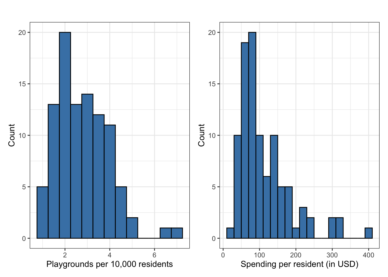
The visualizations and summary statistics for univariate and bivariate exploratory data analysis are in Figure 5.1 and Table 5.1.

(a) Playgrounds per 10,000 residents

(b) Per capita expenditure in USD

Figure 5.1: Univariate exploratory data analysis of playgrounds and per_capita_expend

Table 5.1: Summary statistics of playgrounds and per_capita_spend

Variable	Mean	SD	Min	Q1	Median (Q2)	Q3	Max	Missing
playgrounds	2.8	1.1	1	1.9	2.6	3.6	7	0
per_capita_expend	113.0	72.0	15	65.0	89.0	142.0	399	0

The distribution of playgrounds, the number of playgrounds per 10,000 residents (the response variable), is unimodal and right-skewed. The center of the distribution is the median of about 2.6 playgrounds per 10,000 residents, and the the spread of the middle 50% of the distribution (the IQR) is 1.7. There appear to be two potential outlying cities with more than 6 playgrounds per 10,000 residents, indicating high playground access relative to the other cities in the data set.

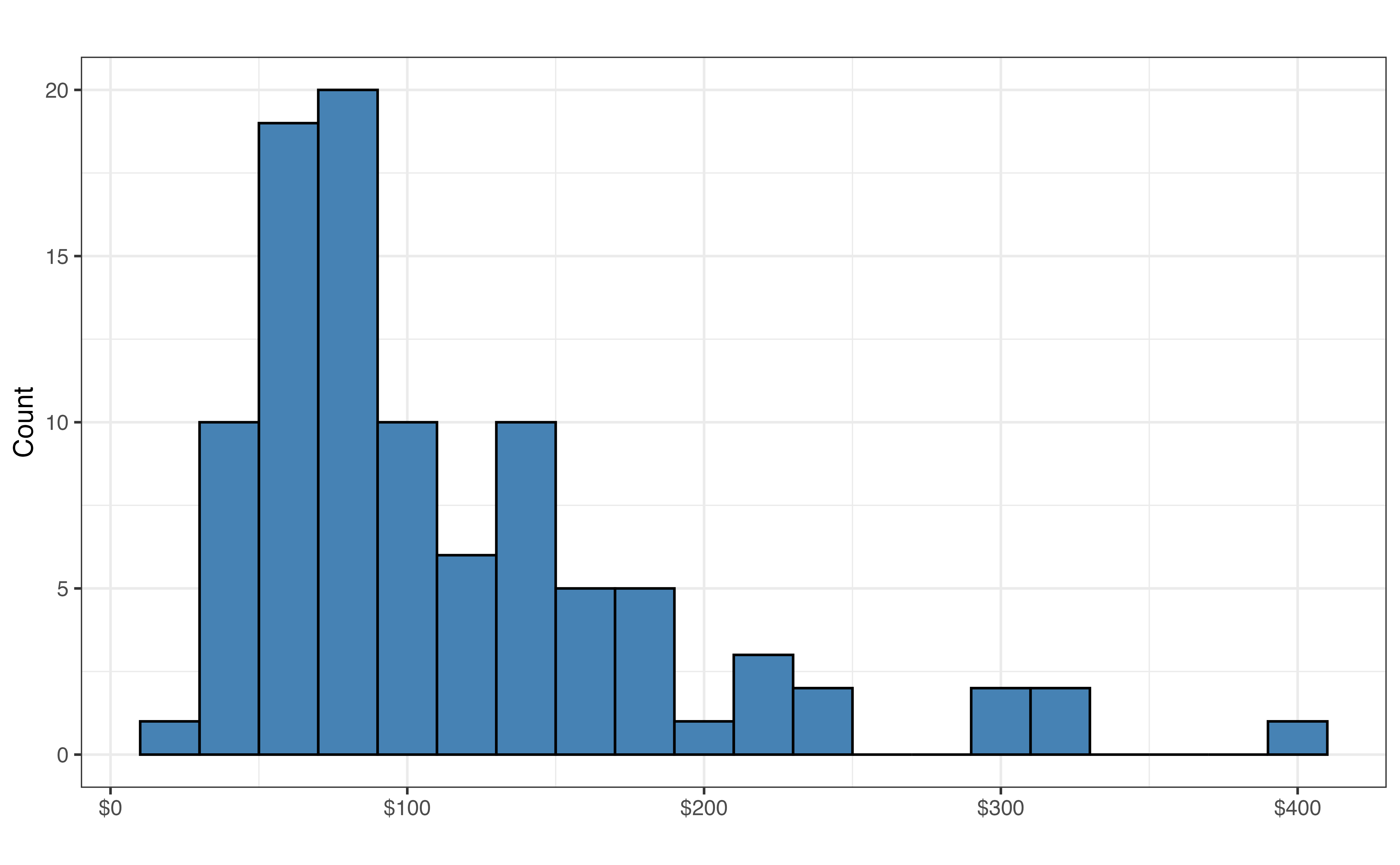
The distribution of per_capita_expend, a city’s expenditure per resident (the predictor variable), is also unimodal and right-skewed. The center of the distribution is around 89 dollars per resident, and the middle 50% of the distribution has a spread of about 77 dollars per resident. Similar to the response variable, there are some potential outliers. There are 5 cities that invests more than 300 dollars per resident.

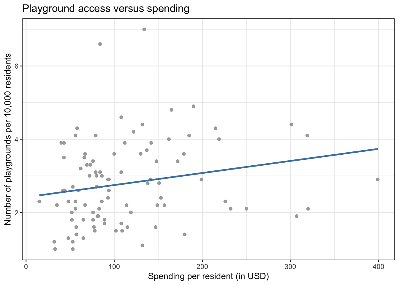
Figure 5.2: Bivariate exploratory data analysis of playgrounds versus per_capita_spend

From Figure 5.2 there appears to be a positive relationship between a city’s per capita expenditure and the number of playgrounds per 10,000 residents. The correlation is 0.206, indicating the relationship between playground access and city expenditure is not strong.This is partially influenced by the outlying observations in that have relatively low values of per capita expenditure but high numbers of playgrounds per 10,000 residents.

Linear regression model

To better explore this relationship, we fit a simple linear regression model of the form

$$\begin{array}{}\text{(5.1)}& \text{playgrounds}={\beta }_0+{\beta }_1\text{per\_capita\_expend}+ϵ,ϵ\sim N(0,{\sigma }_{ϵ}^2)\end{array}$$

The output of the fitted regression model is Table 5.2.

Table 5.2: Linear regression model per_capita_expend and playgrounds

term	estimate	std.error	statistic	p.value
(Intercept)	2.4184	0.2144	11.28	0.0000
per_capita_expend	0.0033	0.0016	2.06	0.0424

$$\begin{array}{}\text{(5.2)}& \widehat{\text{playgrounds}}=2.418+0.003\times \text{per\_capita\_expend}\end{array}$$

• Interpret the slope in the context of the data.
• Does the intercept have a meaningful interpretation? ²

From the sample of 97 cities in 2020, the estimated slope of 0.003. This estimated slope is likely close to but not the exact value of the true population slope we would obtain using data from every city in the United States. Based on the equation alone, we are also not sure if this slope indicates an actual meaningful relationship between the two variables, or if the slope is due to random variability in the data. We will use statistical inference methods to help answer these questions and use the model to draw conclusions about the relationship between per_capita_expend and playgrounds beyond these 97 cities.

5.2 Objectives of statistical inference

Based on the regression output in Table 5.2, for each additional dollar in per capita expenditure, we expect there to be 0.003 more playgrounds per 10,000 residents, on average.

The estimate 0.003 is the “best guess” of the relationship between per capita expenditure and the number of playgrounds per 10,000 residents; however, this is likely not the exact value of the relationship in the population of all US cities. We can use statistical inference, the process of drawing conclusions about the population based on the analysis of the sample data. More specifically, we will use statistical inference to draw conclusions about the population-level slope, ${\beta }_1$.

There are two types of statistical inference procedures:

• Hypothesis tests: Test a specific claim about the population-level slope
• Confidence intervals: A range of values that the population-level slope may reasonably take

This chapter focuses on statistical inference for the slope ${\beta }_1$, but the concepts introduced here can be applied to inference on the population-level intercept ${\beta }_0$ and other population-level parameters.

As we’ll see throughout the chapter, a key component of statistical inference is quantifying the sampling variability, sample-to-sample variability in the statistic that is the “best guest” estimate for the parameter. For example, when we conduct statistical inference on the slope of per capita expenditure ${\beta }_1$, we need to quantify the sampling the variability of the statistic ${\hat{\beta }}_1$, the estimated (sample) slope. This is the amount of variability in ${\hat{\beta }}_1$ that is expected if we repeated the following process many times: (1) collect a new sample that is the same size as our sample data ( 97 in this analysis), and (2) use the new sample to fit a model using per_capita_expend to predict playgrounds to obtain an estimate of the slope. The idea is that ${\hat{\beta }}_1$ would not be the same for each new sample, so we need a way to quantify the variability in these estimated slopes to understand this natural variation. The ${\hat{\beta }}_1$ values from the new samples make up the sampling distribution.

While the process described above would be an approach for constructing the sampling distribution, it is not feasible to collect a lot of new samples in practice. Instead, there are two approaches for obtaining the sampling distribution, in order to quantify the variability in the estimated slopes and conduct statistical inference.

• Simulation-based methods: Quantify the sampling variability by generating a sampling distribution directly from the data

• Theory-based methods: Quantify the sampling variability using mathematical models based on the Central Limit Theorem

Section 5.4 and Section 5.6 introduce statistical inference using simulation-based methods, and Section 5.8 introduces inference using theory-based methods. Before we get into those details, however, let’s introduce more of the foundational ideas underlying simple linear regression and how they relate to statistical inference.

5.3 Foundations of simple linear regression

In Section 4.3.1, we introduced the statistical model for simple linear regression $$\begin{array}{}\text{(5.3)}& Y={\beta }_0+{\beta }_{1}X+ϵϵ\sim N(0,{\sigma }_{ϵ}^2)\end{array}$$

such that $Y$ is the response variable, $X$ is the predictor variable, and $ϵ$ is the error term. Equation 5.3 can be rewritten in terms of the distribution of the response variable $Y$ given the predictor $X$. It is represented as $Y|X$ ( “$Y$ given $X$”)

$$\begin{array}{}\text{(5.4)}& Y|X\sim N({\beta }_0+{\beta }_{1}X,{\sigma }_{ϵ}^2)\end{array}$$

Equation 5.4 is the assumed distribution of the response variable conditional on the predictor variable under the simple linear regression model. Therefore, we conduct simple linear regression assuming Equation 5.4 is true. Based on the equation we specify the assumptions that are made when we do simple linear regression. More specifically, the following assumptions are made based on Equation 5.4:

1. The distribution of the response $Y$ is normal for a given value of the predictor $X$.

2. The expected value (mean) of $Y|X$ is ${\beta }_0+{\beta }_{1}X$. There is a linear relationship between the response and predictor variable.

3. The variance $Y|X$ is ${\sigma }_{ϵ}^2$. This variance is equal for all values of $X$ and thus does not depend on $X$.

4. The error terms for each observation, $ϵ$ in Equation 5.3, are independent. This also means the values of the response variable, and observations more generally, are independent.

Whenever we fit linear regression models and conduct inference on the slope, we do so under the assumption that some or all of these four statements hold. In Chapter 6, we will discuss how to check if these assumptions hold in a given analysis. As we might expect, these assumptions do not always perfectly hold in practice, so we will also discuss circumstances in which an assumption is necessary versus when an assumption can be relaxed. For the remainder of this chapter, however, we will proceed as if all four assumptions hold.

5.4 Bootstrap confidence intervals

We’ll begin by looking at simulation-based methods for statistical inference: bootstrap confidence intervals and permutation tests (Section 5.9.2). In these procedures, we use the sample data to construct a simulated sampling distribution to quantify the sample-to-sample variability in ${\hat{\beta }}_1$. Let’s start with the simulation-based approach to construct confidence intervals.

A confidence interval is a range of values the population-level slope ${\beta }_1$ may reasonably take. Though we have ${\hat{\beta }}_1$, the best guess for the population slope (called a point estimate) , we are more likely to capture the value of the true population slope by computing a range of plausible values than by solely relying on a single estimate. We get this range by constructing $C\mathrm{\%}$ confidence intervals, where $C\mathrm{\%}$ is how confident we are the interval contains ${\beta }_1$ based on the statistical methods.

In order to obtain this range of values we must understand the sampling variability of the statistic. Suppose we repeatedly take samples of size $n$ (the same size as the sample data) and fit regression models to compute ${\hat{\beta }}_1$, the estimated slope. Recall that the sampling variability is the variability in these estimated slopes. In practice, it is generally not feasible to collect multiple samples from the population, so we use our sample data to simulate the process of obtaining new samples. We generate these new samples by bootstrapping, a simulation process in which we generate a sample of size $n$ by sampling with replacement from the current data.

We then fit the regression model and compute ${\hat{\beta }}_1$ for each bootstrap sample. These ${\hat{\beta }}_1$ estimated from the bootstrap samples make up the bootstrap distribution, i.e., the simulated sampling distribution. The variability in this distribution is the sampling variability we need to construct the confidence intervals.

Why do we sample with replacement when generating a bootstrap sample? How would a bootstrap sample compare to the original sample data if sampling is done without replacement?³

5.4.1 Constructing a bootstrap confidence interval for ${\beta }_1$

A bootstrap confidence interval for the population slope, ${\beta }_1$, is constructed using the following steps:

1. Generate $n_{iter}$ bootstrap samples, where $n_{iter}$ is the number of iterations. We typically want to use at least 1000 iterations in order to construct a sampling distribution that is close to the theoretical distribution of ${\hat{\beta }}_1$ defined in Section 5.8.
2. Fit the linear regression model to each of the $n_{iter}$ bootstrap samples to obtain $n_{iter}$ values of ${\hat{\beta }}_1$, the estimated slope. There will also be $n_{iter}$ values of the estimated intercept, ${\hat{\beta }}_0$, but we will ignore those for now because we are not focusing on inference for the intercept.
3. Collect the $n_{iter}$ values of ${\hat{\beta }}_1$ from the previous step to obtain the bootstrapped sampling distribution. It is an approximation of the sampling distribution of ${\hat{\beta }}_1$, and thus provides information about sample-to-sample variability of ${\hat{\beta }}_1$.
4. Use the distribution from the previous step to calculate the $C\mathrm{\%}$ confidence interval. The lower and upper bounds of the interval are the points in the distribution that mark the middle $C\mathrm{\%}$ of the distribution.

Using these four steps, let’s construct the 95% confidence for the population slope ${\beta }_1$ of the relationship between per_capita_spend and playgrounds.

1. Generate 1000 bootstrap samples (97 observations in each sample) by sampling with replacement from the current sample data of 97 observations. The first 10 observations from the first bootstrapped sample are shown in Table 5.3.

Table 5.3: First 10 rows of the first bootstrap sample. The replicate column identifies the bootstrap sample.

replicate	playgrounds	per_capita_expend
1	2.1	320
1	1.8	65
1	2.2	67
1	1.0	33
1	2.6	42
1	2.2	149
1	3.3	73
1	2.2	35
1	1.8	89
1	1.3	65

Why are there 97 observations in each bootstrap sample?⁴

2. Next, we fit a linear model of the form in Equation 5.1 to each of the 1000 bootstrap samples. The estimated slopes and intercepts for the first three bootstrap samples are shown in Table 5.4.

   Table 5.4: Estimated slope and intercept for the first three bootstrap samples.

   replicate	term	estimate
   1	intercept	2.383
   1	per_capita_expend	0.005
   2	intercept	2.545
   2	per_capita_expend	0.002
   3	intercept	2.386
   3	per_capita_expend	0.005

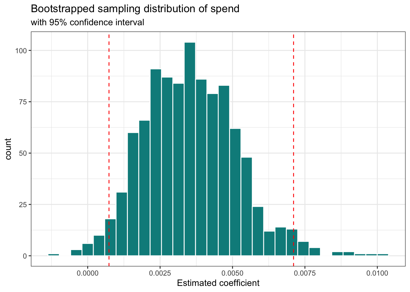
3. We are focused on inference for ${\beta }_1$, the slope of per_capita_expend, so we collect estimated slopes of per_capita_expend to make the bootstrap distribution. This is the approximation of the sampling distribution of ${\hat{\beta }}_1$. A histogram and summary statistics for this distribution are shown in Figure 5.3 and Table 5.5, respectively.

   

   Figure 5.3: Bootstrap distribution of the slope of `per_capita_expend

   Table 5.5: Summary statistics for bootstrap distribution of the slope per_capita_expend

   Min	Q1	Median	Q3	Max	Mean	Std.Dev.
   -0.001	0.002	0.003	0.002	0.01	0.004	0.002

How many values of ${\hat{\beta }}_1$ make up the bootstrap sampling distribution shown in Figure 5.3 and summarized in Table 5.5 ?⁵

4. As the final step, we use the bootstrap distribution to calculate the lower and upper bounds of the 95% confidence interval. These bounds are calculated as the points that mark off the middle 95% of the distribution. These are the points that at the ${2.5}^{th}$ and ${97.5}^{th}$ percentiles, as shown by the vertical lines in Figure 5.4.

Figure 5.4: 95% bootstrap confidence interval for the slope of per_capita_spend

Table 5.6: 95% confidence interval for the slope

Lower bound (2.5th percentile)	Upper bound (97.5th percentile)
0.001	0.007

The 95% bootstrapped confidence interval for ${\beta }_1$, the slope of per_capita_expend is 0.001 to 0.007.

The points at what percentiles in the bootstrap distribution mark the lower and upper bounds for a

• 90% confidence interval?
• 98% confidence interval?⁶

5.4.2 Interpreting the interval

The general interpretation of the 95% confidence interval for ${\beta }_1$, the slope of per_capita_expend is

We are 95% confident that the interval 0.001 to 0.007 contains the population slope for per capita expenditure in the model of the relationship between a city’s per capita expenditure and number of playgrounds per 10,000 residents.

Though this interpretation indicates the range of values that may reasonably contain the true population slope for per_capita_expend, it still requires the reader to further interpret what it means about the relationship between per_capita_expend and playgrounds. It is more informative to interpret the confidence interval in a way that also utilizes the interpretation of the slope from Section 5.1.1 , so the reader more clearly understands what the confidence interval is conveying. Thus, a more complete and informative interpretation of the confidence interval is as follows:

We are 95% confident that for each additional dollar a city spends per resident, there are between 0.001 to 0.007 more playgrounds per 10,000 residents, on average.

This interpretation not only indicates the range of values as before, but it also clearly describes what this range means in terms of the average change in playgrounds per 10,000 residents as a city’s per capita expenditure increases.

5.4.3 What does “confidence” mean?

The beginning of the interpretation for a confidence interval is “We are $C\mathrm{\%}$ confident…”. What does “$C\mathrm{\%}$ confident” mean? The notion of “confidence” refers to the statistical process used construct the confidence interval. This means if we replicate the process thousands of times - obtain a sample of 97 cities, construct a bootstrap distribution for ${\hat{\beta }}_1$, and calculate the bounds that mark the middle $C\mathrm{\%}$ of the distribution, the intervals defined by the upper and lower bounds would contain the value of ${\beta }_1$, the true population slope, $C\mathrm{\%}$ of the time.

In reality we don’t know the value of the population slope (if we did, we wouldn’t need statistical inference!), so we can’t definitively conclude if the interval constructed in Section 5.4.1 is one of the $C\mathrm{\%}$ that contains the population slope or not. Though we aren’t certain that our interval contains the population slope, we can conclude with some level of confidence, $C\mathrm{\%}$ confidence to be exact, that we think it does based on the process.

Thus far, we have used a confidence interval to produce a plausible range of values for the population slope. We can also test specific claims about the population slope using another inferential procedure called hypothesis testing.

5.5 Hypothesis tests

Hypothesis tests are used to evaluate a claim about about a population parameter. The claim could be based on previous research, an idea a research or business team wants to explore, or a general statement about the parameter. We will again focus on the population slope ${\beta }_1$. Before getting into the details of simulation-based hypothesis tests, we’ll describe the steps for a hypothesis test based on a commonly used analogy, the general procedure of a court trial in the United States (US) judicial system.

5.5.1 Define the hypotheses

The first step of any hypothesis test (or trial) is to define the hypotheses that will be evaluated. These hypotheses are called the null and alternative. The null hypothesis $(H_0)$ is the baseline condition typically indicating no relationship between the response and predictor, and the alternative hypothesis $(H_a)$ is defined by the claim being tested. Typically, the claim is that there is some relationship between the two variables.

In the US judicial system, a defendant is deemed innocent unless proven otherwise. Therefore, the null and alternative hypotheses are $H_0$: the defendant is not guilty, and $H_a$: the defendant is guilty. We say that a person is “innocent until proven guilty beyond a reasonable doubt.” Therefore, the trial proceeds assuming the null hypothesis of innocence is true and the objective is to evaluate the strength of evidence against this hypothesis. The same is true for hypothesis testing in statistics. The test is conducted under the assumption that the null hypothesis, $H_0$, is true, and we use statistical methods to evaluate the strength of the evidence against $H_0$.

5.5.2 Evaluate the evidence

The primary component of trial (or hypothesis test) is a presenting and evaluating the evidence. In a trial, this is the point when the evidence is presented and it is evaluated under the assumption the null hypothesis (defendant is not guilty) is true. Thus, the lens in which the evidence is being evaluated is “given the defendant is not guilty, how likely is it that this evidence would exist?”

For example, suppose an individual is on trial for a robbery at a jewelry store. The null hypothesis is that they are not guilty and did not rob the jewelry store. The alternative hypothesis is they are guilty and did rob the jewelry store. If there is evidence that the person was in a different city during the time of the jewelry store robbery, the evidence would be more in support of the null hypothesis of innocence. It seems plausible the individual could have been in a different city at the time of the robbery if the null hypothesis is true. Alternatively, if some of the missing jewelry was found in the individual’s car, the evidence would seem to be strongly in support of the alternative hypothesis. If the null hypothesis is true, it does not seem likely that the individual would have the missing jewelry in their car.

In hypothesis testing, the “evidence” being assessed is the analysis of the sample data. Thus we are considering the question “given the null hypothesis is true, how likely is it to observe the results seen in the sample data?” We will introduce approaches to address this question using simulation-based methods in Section 5.6 and theory-based methods in Section 5.8.3.

5.5.3 Make a conclusion

There are two typical conclusions in a trial in the US judicial system - the defendant is guilty or not guilty based on the evidence. The criteria to conclude the alternative that a defendant is guilty is that the strength of evidence must be “beyond reasonable doubt”. If there is sufficiently strong evidence against the null hypothesis of not guilty, then the conclusion is the alternative hypothesis that the defendant is guilty. Otherwise, the conclusion is that the defendant is not guilty, indicating the evidence against the null was not strong enough to otherwise refute it. Note that this is the not the same as “accepting” the null hypothesis but rather indicating that there wasn’t enough evidence to suggest otherwise.

Similarly in hypothesis testing, we will use a predetermined threshold to assess if the evidence against the null hypothesis is strong enough to reject the null hypothesis and conclude the alternative, or if there is not enough evidence “beyond a reasonable doubt” to draw a conclusion other than the assumed null hypothesis.

5.6 Permutation tests

Now that we have explained the general process of hypothesis testing, let’s take a look at hypothesis testing using a simulation-based approach, called a permutation test.

The four steps of permutation test for a slope ${\beta }_1$ are

1. State the null and alternative hypotheses.
2. Generate the null distribution.
3. Calculate the p-value.
4. Draw a conclusion.

These steps are described in detail in the context of the hypothesis test for the slope in Equation 5.1.

5.6.1 State the hypotheses

As defined in Section 5.5 the null hypothesis ($H_0$) is the baseline condition, and the alternative hypothesis ($H_a$) is defined by the claim being tested. Recall from Section 5.1 that one objective for the analysis in this chapter is to investigate whether per capita expenditure is useful in understanding variability in playground access in US cities. In terms of the linear regression model, the claim being tested is whether there is a linear relationship between per_capita_expend and playgrounds. The null hypothesis is the baseline condition of there being no linear relationship between the two variables. We use this claim to define the alternative hypothesis.

• Null hypothesis: There is no linear relationship between playgrounds per 10,000 residents and per capita expenditure. The slope of per_capita_expend is equal to 0. $(H_0:{\beta }_1=0)$
• Alternative hypothesis: There is a linear relationship between playgrounds per 10,000 residents and per capita expenditure. The coefficient of per_capita_expend is not equal to 0. $(H_a:{\beta }_1\ne 0)$
  • Note that we have not hypothesized whether the slope is positive or negative.

The hypotheses are defined specifically in terms of the linear relationship between the two variables, because we are ultimately drawing conclusions about the slope ${\beta }_1$.

Mathematical statement of hypotheses for ${\beta }_1$

Suppose there is a response variable $Y$ and a predictor variable $X$ such that

$$Y={\beta }_0+{\beta }_{1}X+ϵ,ϵ\sim N(0,{\sigma }_{ϵ}^2)$$

The hypotheses for testing whether there is a linear relationship between $X$ and $Y$ in the population are

$$\begin{array}{}\text{(5.5)}& \begin{array}{rl}& H_0:{\beta }_1=0\\ & H_a:{\beta }_1\ne 0\end{array}\end{array}$$

One vs. two-sided hypotheses

The alternative hypothesis defined in Equation 5.5 is “not equal to 0”. This is the alternative hypothesis corresponding to a two-sided hypothesis test, because it includes the scenarios in which ${\beta }_1$ is less than or greater than 0. There are two other options for defining the alternative hypothesis, “${\beta }_1$ is less than 0” ($H_a:{\beta }_1<0$) and “${\beta }_1$ is greater than 0” ($H_a:{\beta }_1>0$). These are one-sided hypothesis tests, as they only consider the alternative scenario in which ${\beta }_1$ is either less than or greater than 0, respectively.

A one-sided hypothesis test imposes some information about the direction of the parameter, that is positive ($>0$) or negative ( $<0$). Given this additional information imposed by the direction of the alternative hypothesis, it requires less evidence to reject the null hypothesis in favor of the alternative. Therefore, it is best to use a one-sided hypothesis only if (1) there is some indication from previous knowledge or research that the relationship between the response variable and the predictor variable is in a particular direction, or (2) only one direction of the relationship between the response and predictor variables is relevant in practice. Outside of these two scenarios, it is not advisable to use the one-sided hypothesis, as there could appear to be a statistically significant relationship between the two variables merely by chance of how the hypotheses were constructed.

Because a two-sided hypothesis test makes no assumption about the direction of the relationship between the response variable and predictor variable. It is a good starting point for drawing conclusions about the relationship between the two variables. From the two-sided hypothesis, we will conclude whether there is or is not sufficient statistical evidence of a linear relationship between the response and predictor. With this conclusion, we cannot determine if the relationship between the variables is positive or negative without additional analysis. We use a confidence interval (Section 5.4) to make specific conclusions about the direction and magnitude of the relationship.

5.6.2 Simulate the null distribution

Recall that hypothesis tests are conducted assuming the null hypothesis $H_0$ is true. Based on the hypotheses defined in Section 5.6.1, a hypothesis test for the slope is conducted under the assumption ${\beta }_1=0$ , that there is no linear relationship between the response and predictor variables.

To assess the evidence, we will use a simulation-based method to approximate the sampling distribution of the estimated slope ${\hat{\beta }}_1$ under the assumption that $H_0:{\beta }_1=0$ is true. This distribution, called the null distribution, allows us to understand the sample-to-sample variability under the scenario in which the true population slope equals 0. The variability in the simulated null distribution will be the same (or very similar since we are working with simulated data) as the variability in the bootstrap distribution, but the difference between the two distributions is the location of the center. The center for the bootstrap distribution in Section 5.4 is close to the value of ${\hat{\beta }}_1$ estimated from the data. The center of the null distribution, however, is the null hypothesized value of 0. Therefore, to construct the null distribution for hypothesis testing, we will use a different simulation method, called permutation sampling.

In permutation sampling the values of the predictor variable are randomly shuffled and paired with values of the response, thus generating a new sample of the same size as the original data. The process of randomly pairing the values of the response and the predictor variables simulates the null hypothesized condition that there is no linear relationship between the two variables.

The steps for simulating the null distribution using permutation sampling are the following:

1. Generate $n_{iter}$ permutation samples, where $n_{iter}$ is the number of iterations. We ideally use at least 1,000 iterations in order to construct a distribution that is close to the theoretical null distribution defined in Section 5.8.
2. Fit the linear regression model to each of the $n_{iter}$ permutation samples to obtain $n_{iter}$ values of ${\hat{\beta }}_1$, the estimated slope. There will also be $n_{iter}$ values of ${\hat{\beta }}_0$ the estimated intercepts; we will ignore those for now because we are focused on inference for the slope.
3. Collect the $n_{iter}$ values of ${\hat{\beta }}_1$ from the previous step to make the simulated null distribution. This is an approximation of the distribution of ${\hat{\beta }}_1$ values if we were to repeatedly take samples the same size as the original data and fit the linear regression model to each sample, under the assumption that the null hypothesis is true.

Let’s simulate the null distribution to test the hypotheses in Equation 5.5 for the parks data.

1. First we generate 1,000 permutation samples, such that in each sample, we permute the values of per_capita_expend, randomly pairing each to a value of playgrounds. This is to simulate the scenario in which there is no linear relationship between per_capita_expend and playgrounds. The first 10 rows of the first permutation sample are in Table 5.7.

Table 5.7: First 10 rows of the first permutation sample. The replicate column identifies the permutation sample.

replicate	playgrounds	per_capita_expend
1	2.1	319
1	1.8	307
1	2.2	219
1	1.0	301
1	2.6	190
1	2.2	250
1	3.3	215
1	1.8	399
1	1.8	162
1	1.9	179

2. Next, we fit a linear regression model to each of the 1000 permutation samples. This gives us 1000 estimates of the slope and intercept. The slopes estimated from the first 10 permutation samples are shown in Table 5.8.

Table 5.8: Estimated slopes from first 10 permutation samples.

replicate	term	estimate
1	per_capita_expend	0.000
2	per_capita_expend	0.001
3	per_capita_expend	0.001
4	per_capita_expend	-0.002
5	per_capita_expend	-0.002
6	per_capita_expend	0.004
7	per_capita_expend	-0.002
8	per_capita_expend	-0.002
9	per_capita_expend	-0.001
10	per_capita_expend	0.001

3. Next, we collect the estimated slopes from the previous step to construct the simulated null distribution. We will use this distribution to assess the strength of the evidence from the original sample data against the null hypothesis.

   

   Figure 5.5: Simulated null distribution to test the slope of per_capita_expend

Table 5.9: Summary statistics of the simulated null distribution to test the slope of per_capita_expend

Min	Q1	Median	Q3	Max	Mean	Std.Dev.
-0.005	-0.001	0	-0.001	0.006	0	0.002

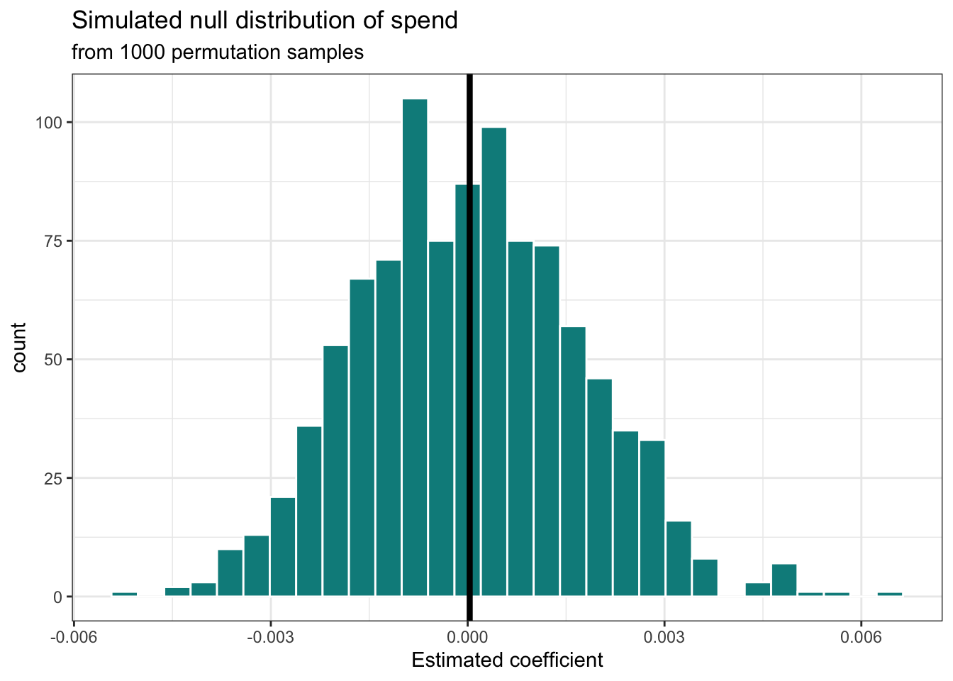
Note that the distribution visualized in Figure 5.5 and summarized in Table 5.9 is approximately unimodal, symmetric, and looks similar to the normal distribution. As the number of iterations (permutation samples) increases, the simulated null distribution will be closer and closer to a normal distribution. Additionally, the center of the distribution is approximately 0, the null hypothesized value. The standard deviation of this distribution 0.002 is an estimate of the standard error of ${\hat{\beta }}_1$, the sample-to-sample variability in the estimates of ${\hat{\beta }}_1$ when taking random samples of size 97, the same size as the original data.

How does the estimated variability in the simulated null distribution in Table 5.9 compare to the variability in the bootstrapped distribution in Table 5.5? Is this what you expected? Why or why not?⁷

5.6.3 Calculate p-value

The null distribution helps us understand the values ${\hat{\beta }}_1$, the slope of per_capita_expend, is expected to take if we repeatedly take random samples and fit a linear regression model, assuming the null hypothesis ${\beta }_1=0$ is true. To evaluate the strength of evidence against the null hypothesis, we will compare the estimated slope in Table 5.2, ${\hat{\beta }}_1=$ 0.003 (the evidence) to what we would expect ${\hat{\beta }}_1$ to be based on the null distribution.

This comparison is quantified using a p-value. The p-value is the probability of observing estimated slopes at least as extreme as the value estimated from the sample data, given the null hypothesis is true. In the context of the parks data, the p-value is the probability of observing values of the slope that are at least as extreme as ${\hat{\beta }}_1=$ 0.003 in the null distribution.

In the context of statistical inference, the phrase “more extreme” means the area between the estimated value ( ${\hat{\beta }}_1$ in our case), and the outer tail(s) of the simulated null distribution. The alternative hypothesis determines which tail(s) to include when calculating the p-value.

• If $H_a:{\beta }_1>0$, the p-value is the probability of obtaining a value in the null distribution that is greater than or equal to ${\hat{\beta }}_1$.

• If $H_a:{\beta }_1<0$, the p-value is the probability of obtaining a value in the null distribution that is less than or equal to ${\hat{\beta }}_1$.

• If $H_a:{\beta }_1\ne 0$, the p-value is the probability of obtaining a value in the null distribution whose absolute value is greater than or equal to ${\hat{\beta }}_1$ . This includes values that are greater than or equal to $|{\hat{\beta }}_1|$ or less than or equal to $-|{\hat{\beta }}_1|$.

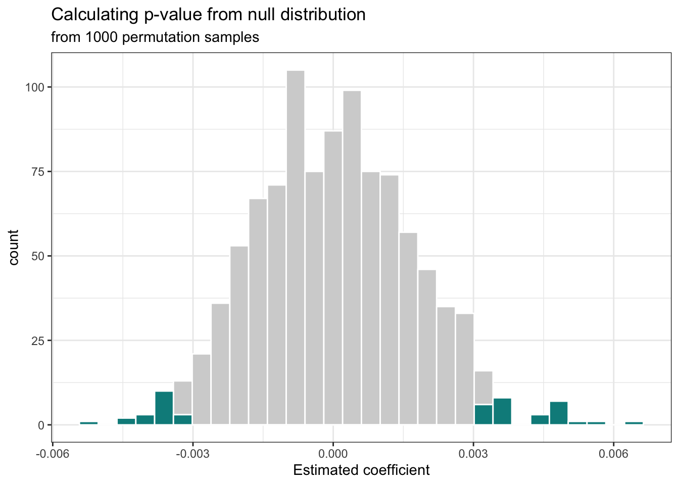
Recall from Section 5.6.1 that we are testing a two-sided alternative hypothesis. Therefore, we will calculate the p-value corresponding to the alternative hypothesis $H_a:{\beta }_1\ne 0$. As illustrated in Figure 5.6, this p-value is the probability of observing the slope that is 0.003 or more extreme, given the null hypothesis is true. In this case, it is the probability of observing a value in the null distribution that is greater than or equal to |0.003| or a value that is less than or equal to -|0.003|.

The p-value for this hypothesis test is 0.046 and is shown by the dark shaded area in Figure 5.6.

Figure 5.6: Simulated null distribution with p-value represented by the shaded area. The shaded area are values less than -0.003 and greater than 0.003.

Use the definition of the p-value at the beginning of this section to interpret the p-value of 0.046 in the context of the data.⁸

5.6.4 Draw conclusion

We ultimately want to evaluate the strength of evidence against the null hypothesis. The p-value is a measure of the strength of that evidence and is used to draw one of the following conclusions:

• If the p-value is “sufficiently small”, there is strong evidence against the null hypothesis. We reject the null hypothesis, $H_0$, and conclude the alternative $H_a$.
• If the p-value is not “sufficiently small”, there is not strong enough evidence against the null hypothesis. We fail to reject the null hypothesis, $H_0$, and stay with the null hypothesis.

We use a predetermined decision-making threshold called an $\mathit{\alpha }$-level to determine if a p-value is sufficiently small enough to reject the null hypothesis.

• If $\text{p-value}<\alpha$, then reject $H_0$

• If $\text{p-value}\ge \alpha$, then fail to reject $H_0$.

A commonly used threshold is $\alpha =0.05$. If stronger evidence is required to reject the null hypothesis, then a lower threshold can be used to make a conclusion. If such strong evidence is not required (this may be the case in analyses with very small sample sizes), then a threshold can be used. It is general convention to use a threshold 0.1 or less, so any p-value 0.1 is considered large enough to fail to reject the null hypothesis.

Back to the parks analysis. We will use the common threshold of $\alpha =0.05$.

The p-value calculated in the previous section is 0.046. Therefore, we reject the null hypothesis $H_0$. The data provide sufficient evidence of a linear relationship between the amount a city spends per resident and the number of playgrounds per 10,000 residents.

5.6.5 Type I and Type II error

Regardless of the conclusion that is drawn (reject or fail to reject the null hypothesis), we have not determined that the null or alternative hypothesis are definitive truth. We have just concluded that the evidence (the data) has provided more evidence in favor of one conclusion versus the other. As with any statistical procedure, there is the possibility of making an error, more specifically a Type I or Type II error. Because we don’t know the value of the population slope, we will not know for certain whether we have made an error; however, understanding the potential errors that can be made can help inform the decision-making threshold $\alpha$ and make a more informed assessment about the implication of these results in practice.

Table 5.10 shows how Type I and Type II errors correspond to the (unknown) truth and the conclusion drawn from the hypothesis test.

Table 5.10: Type I and Type II error

		Truth
		$H_0$ true	$H_a$ true
Hypothesis test decision	Fail to reject $H_0$	Correct decision	Type II error
	Reject $H_0$	Type I error	Correct decision

A Type I error has occurred if the null hypothesis is actually true, but the p-value is small enough to reject the null hypothesis. The probability of making this type of error is the decision-making threshold $\alpha$. This is because $P(\text{reject }{H}_0|H_0\text{ true})=\alpha$, meaning the probability of rejecting the null hypothesis given the null is true is $\alpha$.

A Type II error has occurred if the alternative hypothesis is actually true, but we fail to reject the null hypothesis, because the p-value is large. Computing the probability of making this type of error is less straightforward. It is calculated as $1-Power$ , where the $Power=P(\text{reject }{H}_0|H_a\text{ true})$.

In the context of the parks data, a Type I error is concluding that there is a linear relationship between per capita expenditure and playgrounds per 10,000 residents in the model, when there actually isn’t one in the population. A Type II error is concluding there is no linear relationship between per capita expenditure and playgrounds per 10,000 residents when in fact there is.

Given the conclusion in Section 5.6.4, is it possible we’ve made a Type I or Type II error?⁹

5.7 Relationship between confidence intervals and hypothesis tests

At this point, we might wonder whether there is any connection between the confidence intervals and hypothesis tests. Spoiler alert: there is!

Testing a claim with the two-sided alternative $H_a:{\beta }_1\ne 0$ and decision-making threshold $\alpha$ is equivalent to using the $C\mathrm{\%}$ confidence interval to evaluate the claim, where $C=(1-\alpha )\times 100$. This means we can also use confidence intervals to evaluate two-sided hypotheses. When using a confidence interval to draw conclusions about a claim, we use the following guide:

• If the null hypothesized value ( $0$ based on the tests defined in Section 5.6.1 ) is within the range of the confidence interval, fail to reject $H_0$ at the $\alpha$-level.

• If the null hypothesized value is not within the range of the confidence interval, reject $H_0$ at the $\alpha$-level.

This illustrates the power of confidence intervals; they can not only be used to draw a conclusion about a claim (reject or fail to reject $H_0$), but they also give the range values that the population slope may take. Thus, it is good practice to always report the confidence interval, because the confidence interval provides more detail about a population slope ${\beta }_1$ beyond the reject/fail to reject conclusion of the hypothesis test.

When we reject a null hypothesis, we conclude that there is a statistically significant linear relationship between the response and predictor variables. Concluding there is statistically significant relationship between the response and predictor, however, does not necessarily mean that the relationship is practically significant. The practical significance, how meaningful the results are in the real world, is determined by the magnitude of the estimated slope of the predictor on the response and what an effect of that magnitude means in the context of the data and analysis question.

5.8 Theory-based inference

Thus far we have approached inference using simulation-based methods (bootstrapping and permutation) to generate sampling distributions and null distributions. When certain conditions are met, however, we can use theoretical results about the sampling distribution to understand the variability in ${\hat{\beta }}_1$. In this section, we present that theory, then use it to conduct statistical inference for the population slope. Notice as we go through this section is that the inferential procedures and conclusions are very similar as before. The primary difference is in how we understand the sampling variability in ${\hat{\beta }}_1$ and obtain the null distribution.

5.8.1 Central Limit Theorem

The Central Limit Theorem (CLT) is a foundational theorem in statistics about the distribution of a statistic and the associated mathematical properties of that distribution. For the purposes of this text, we will focus on what the Central Limit Theorem says the distribution of an estimated slope ${\hat{\beta }}_1$, but note that this theorem applies to statistics other than the slope. We will also focus on the results of the theorem and less so on derivations or advanced mathematical details of the Central Limit Theorem.

By the Central Limit Theorem, we know under certain conditions (more on these conditions in the Chapter 6) $$\begin{array}{}\text{(5.6)}& {\hat{\beta }}_1\sim N({\beta }_1,S{E}_{{\hat{\beta }}_1})\end{array}$$

Equation 5.6 means that by the Central Limit Theorem, we know that the sampling distribution of ${\hat{\beta }}_1$ is (1) normal, (2) with a expected value at the true slope ${\beta }_1$, and (3) a standard error of $S{E}_{{\hat{\beta }}_1}$¹⁰. The center of this distribution ${\beta }_1$ is unknown; the purpose of statistical inference is to draw conclusions about ${\beta }_1$. The standard error of this distribution $S{E}_{{\hat{\beta }}_1}$ is

$$\begin{array}{}\text{(5.7)}& S{E}_{{\hat{\beta }}_1}={\hat{\sigma }}_{ϵ}\sqrt{\frac{1}{(n-1)s_X^2}}\end{array}$$

where $n$ is the number of observations, $s_X^2$ is the variance of the predictor variable $X$, and ${\hat{\sigma }}_{ϵ}$ is the regression standard error, the variability of the observations around the regression line. The regression error is introduced in more detail in Section 5.8.2. The details of how this formula is derived is beyond the scope of this text, but let’s take a moment to think about what we know about the sampling variability of ${\hat{\beta }}_1$ from Equation 5.7.

The regression standard error ${\hat{\sigma }}_{ϵ}$ is in the numerator, indicating one would expect more variability in ${\hat{\beta }}_1$ when there is more variability in the data about the regression line. The variability in the predictor variable $s_X^2$ is in the denominator, indicating we expect more variability in ${\hat{\beta }}_1$ when there is less variability in the values of the predictor. Therefore, $S{E}_{{\hat{\beta }}_1}$ is the balance between the variability about the regression line and the variability in the predictor variable itself.

As you will see in the following sections, we will use this estimate of the sampling variability in the estimated slope to draw conclusions about the true relationship between the response and predictor variables based on hypothesis testing and confidence intervals.

5.8.2 Estimating ${\sigma }_{ϵ}$

As discussed in Section 4.3.1, there are three parameters that need to be estimated for simple linear regression ${\beta }_0$, ${\beta }_1$, and ${\sigma }_{ϵ}$. Section 4.4 introduced least squares regression, a method for deriving ${\hat{\beta }}_0$ and ${\hat{\beta }}_1$ the estimates for intercept and slope, respectively. Now, we turn to the estimation of ${\sigma }_{ϵ}$, also known as the regression standard error.

By obtaining the estimates ${\hat{\beta }}_0$ and ${\hat{\beta }}_1$, we have the equation of the regression line and therefore can estimate the expected value $Y$ given a value of the predictor $X$. We can then use the residuals ($e_i=y_i-{\hat{y}}_i$) to estimate the variability of the distribution of the response variable about the regression line (see Section 5.3). The regression standard error is the estimate of this variability as it is the estimated standard deviation of the distribution of the errors (Equation 5.3). The equation for the regression standard error is shown in Equation 5.8 ¹¹.

$$\begin{array}{}\text{(5.8)}& {\hat{\sigma }}_{ϵ}=\sqrt{\frac{\sum _{i=1}^n{e}_i^2}{n-2}}=\sqrt{\frac{\sum _{i=1}^n(y_i-{\hat{y}}_i{)}^2}{n-2}}\end{array}$$

You may have noticed that the denominator in Equation 5.8 is $n-2$ not $n$ or $n-1$. The value $n-2$ is called the degrees of freedom (df). The degrees of freedom are how many observations are available to understand variability about the regression line. We need at a minimum two observations to estimate the equation for the simple linear regression line, i.e., it takes at a minimum two points to make a line. The remaining $n-2$ observations help us understand variability about the line. We will talk more about how we use degrees of freedom as we define the distribution used to compute confidence intervals and conduct hypothesis tests.

Recall that the standard deviation is the average distance between each observation and the mean of the distribution. Similarly, the regression standard error can be thought of as the average distance the observed value the response is from the regression line. The regression standard error ${\hat{\sigma }}_{ϵ}$ is used to quantify the sampling variability in the estimated slope ${\hat{\beta }}_1$ (Equation 5.7), so we will use this value as we conduct inference on the slope.

5.8.3 Hypothesis test for the slope

The overall goals of hypothesis tests for a population slope are the same when using theory-based methods as previously described in Section 5.5. We define a null and alternative hypothesis, conduct testing assuming the null hypothesis is true, and draw a conclusion based on an evaluation of the strength of evidence against the null hypothesis. The main difference from the simulation-based approach in Section 5.6 is in how we quantify the variability in ${\hat{\beta }}_1$ and thus obtain the null distribution. In Section 5.6.2 we used permutation sampling to generate the null distribution. We’ll see that by the Central Limit Theorem we have results that specify exactly how the null distribution is defined.

The steps for conducting a hypothesis test based on the Central Limit Theorem are the following:

1. State the null and alternative hypotheses.
2. Calculate a test statistic.
3. Calculate a p-value.
4. Draw a conclusion.

As in Section 5.6 the goal is to use hypothesis testing to determine whether there is evidence of a statistically significant linear relationship between a response and predictor variable, corresponding to the two-sided alternative hypothesis of “not equal to 0”. Therefore, the null and alternative hypotheses are the same as defined in Equation 5.5 $$\begin{array}{r}{H}_0:{\beta }_1=0\\ H_a:{\beta }_1\ne 0\end{array}$$

The next step is to calculate a test statistic. Similar to a $z$-score in the Normal distribution, the test statistic tells us how far the observed slope is from the hypothesized center of the distribution. The general form of a test statistic is

$$T=\frac{\text{estimate }-\text{ hypothesized}}{\text{standard error}}$$

More specifically, in the hypothesis test for ${\beta }_1$, the test statistic is

$$\begin{array}{}\text{(5.9)}& T=\frac{{\hat{\beta }}_1-0}{S{E}_{{\hat{\beta }}_1}}\end{array}$$

To calculate the test statistic, the estimated slope is shifted by the mean, and then rescaled by the standard error. Let’s consider what we learn from the test statistic. Recall that by the Central Limit Theorem, the distribution of ${\hat{\beta }}_1$ is $N({\beta }_1,S{E}_{{\hat{\beta }}_1})$. Because we conduct hypothesis testing under the assumption the null hypothesis is true, we are assuming that the mean of this distribution of ${\beta }_1=0$.

Since the hypothesized mean is ${\beta }_1=0$, we shift by 0 and rescale by $S{E}_{{\hat{\beta }}_1}$, defined in Equation 5.7. Thus, the test statistic is the number of standard errors the estimated slope is from the hypothesized mean of the sampling distribution. The magnitude of the test statistic $|T|$ provides a measure of how far the observed slope is from the center of the distribution, and the sign of $T$ indicates whether the observed slope is above (positive sign) or below (negative sign) the hypothesized mean of 0.

Consider the magnitude of the test statistic, $|T|$. Do you think test statistics with small magnitude provide evidence in support or against the null hypothesis? What about test statistics with large magnitude?¹²

Next, we use the test statistic to calculate a p-value and we will ultimately use the p-value to draw a conclusion about the strength of the evidence against the null hypothesis, as before. The test statistic, $T$, follows a $t$ distribution with $n-2$ degrees of freedom, denoted as $T\sim t_{n-2}$ . Similar to the simulated null distribution in Section 5.6.2, we use this $t_{n-2}$ distribution to evaluate how far the estimated slope is from what we would expect given the null hypothesis is true.

Though the sampling distribution of ${\hat{\beta }}_1$ is normal by the Central Limit Theorem (Equation 5.6), the test statistic follows a $t$ distribution. The $t$ distribution is used, because the value $S{E}_{{\hat{\beta }}_1}$ in the test statistic is calculated using the regression standard error, ${\hat{\sigma }}_{ϵ}$ (see Equation 5.7) We know the estimates ${\hat{\sigma }}_{ϵ}$ and $S{E}_{{\hat{\beta }}_1}$ are likely not equal to the true population values, so we need a distribution that allows for a bit more variability when calculating the p-value. The $t$ distribution better accounts for this extra variability compared to the standard normal distribution.

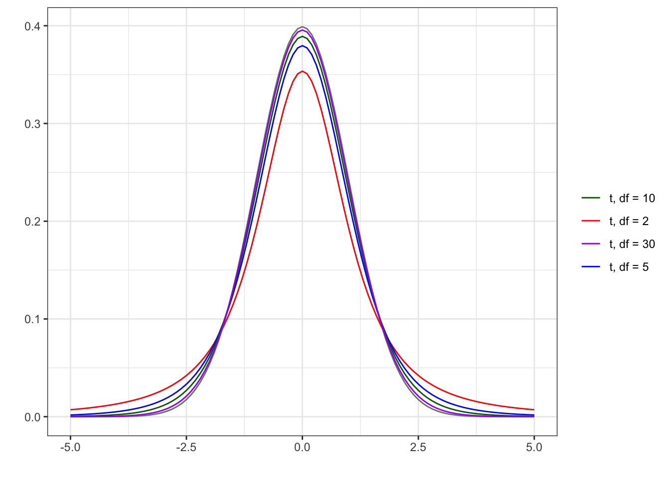
Figure 5.7 shows the standard normal distribution $N(0,1)$ and the $t$ distribution for different degrees of freedom. The $t$ distribution is very similar to the standard normal distribution: they are both centered at 0 and have a shape that is unimodal and symmetric. In other words, they both look like “bell curves” centered at 0. The difference is that the $t$ distribution allows for more variability than what is expected in the standard normal distribution. This is also referred to as having “heavier tails”. The $t$ distribution has more area under the curve in the tails (or more extreme values) of the distribution, meaning that more extreme values are more likely under the $t$ distribution than under the $N(0,1)$ distribution. This is most clearly seen by th comparing the height of tails for $t_2$ and $N(0,1)$. As the degrees of freedom increase, the $t$ distribution becomes closer to the the standard normal distribution.

Figure 5.7: Standard normal vs. t distributions

As described in Section 5.6.3, because the alternative hypothesis is “not equal to”, the p-value is calculated on both the high and low extremes of the distribution as shown in Equation 5.10.

$$\begin{array}{}\text{(5.10)}& \begin{array}{rl}& \text{p-value}=Pr(|t|>|T|)=Pr(t<-|T|\text{ or }t>|T|)\\ & \text{where }t\sim t_{n-2}\end{array}\end{array}$$

We compare the p-value to a decision-making threshold $\alpha$ to draw final conclusions. If $\text{p-value}<\alpha$ , we reject the null hypothesis and conclude the alternative. Otherwise, we fail to reject the null hypothesis. See Section 5.6.4 for more detail about using the $\alpha$-level and p-value to draw conclusions.

Now let’s apply this process to test whether there is evidence of a linear relationship between per capita expenditure and the number of playgrounds per 10,000 residents. As before, the null and and alternative hypotheses are

$$\begin{array}{rl}& H_0:{\beta }_1=0\\ & H_a:{\beta }_1\ne 0\end{array}$$

where ${\beta }_1$ is the true slope between per_capita_expend and playgrounds. The observed slope from Table 5.2, we know the observed slope ${\hat{\beta }}_1$ is 0.003 and the estimated standard error $S{E}_{{\hat{\beta }}_1}$ is 0.002. The test statistic is

$$T=\frac{0.0033-0}{0.0016}=2.063$$

This test statistic means that assuming the true slope of per_capita_expend in this model is 0 and thus the mean of the distribution of ${\hat{\beta }}_1$ is 0, the observed slope of 0.003 is 2.063 standard errors above this hypothesized mean. It’s difficult to determine whether or not this is really “far enough” away from the center of the distribution, but we can calculate a p-value to determine the probability of observing a slope at least this far given the null hypothesis is true.

Given there are $n$ = 97 observations, the test statistic follows a $t$ distribution with $97-2=$ 95 degrees of freedom. The p-value, is $Pr(t<-|2.063|\text{ or }t>|2.063|)=$ 0.042.

Using a decision-making threshold $\alpha =0.05$, the p-value $0.042$ is sufficiently small, so we reject the null hypothesis. The data provide sufficient evidence that the coefficient of per_capita_expend is not 0 in this model and that there is a statistically significant linear relationship between a city’s per capita expenditure and playgrounds per 10,000 residents in US cities.

Note that this conclusion is the same as in Section 5.6.4 using a simulation-based approach (even with small differences in the p-value). This is what we would expect, given these are the two different approaches for conducting the same inferential process. We are also conducting the tests under the same assumptions that the null hypothesis is true. The difference is in the methods available to quantify $S{E}_{{\hat{\beta }}_1}$, simulation-based versus theory-based.

5.8.4 Confidence interval

As with simulation-based inference, a confidence interval calculated based on the results from the Central Limit Theorem is an estimated range of the values that ${\beta }_1$ can reasonably take. The purpose, interpretation, and conclusions drawn from confidence intervals are the same as described before in Section 5.4. What differs, however, is how the interval is calculated. In simulation-based inference, we used bootstrapping to construct a sampling distribution to understand sample-to-sample variability in ${\beta }_1$. By the Central Limit Theorem, we know exactly how to quantify the sample-to-sample variability in ${\hat{\beta }}_1$ using theoretical results.

The equation for a $C\mathrm{\%}$ confidence interval for ${\beta }_1$ is

$$\begin{array}{}\text{(5.11)}& {\hat{\beta }}_1\pm t^{\ast }\times S{E}_{{\hat{\beta }}_1}\end{array}$$

where $t^{\ast }\sim t_{n-2}$.

In Section 5.8.1, we discussed ${\hat{\beta }}_1$ and its standard error $S{E}_{{\hat{\beta }}_1}$. Now we’ll focus on $t^{\ast }$, known as the critical value.

The critical value is the point on the $t_{n-2}$ distribution such that the probability of being between $-t^{\ast }$ and $t^{\ast }$ is $C\mathrm{\%}$. Thinking about this visually, this is the point such that the $C\mathrm{\%}$ of the area under the curve is between $-t^{\ast }$ and $t^{\ast }$. Note that we are still using a $t$ distribution with $n-2$ degrees of freedom, the same distribution used to calculate the p-value in the hypothesis tests. The critical value can be calculated from modern statistical software or using online apps (more on this in Section 5.9.3).

Let’s calculate the 95% confidence interval for the slope of per_capita_spend. There are 97 observations, so we use the $t$ distribution with 95 degrees of freedom. The critical value on the $t_{95}$ distribution is 1.985. Plugging these values into Equation 5.11, the 95% confidence interval is

$$\begin{array}{}\text{(5.12)}& \begin{array}{r}0.0033\pm 1.985\times 0.0016\\ 0.0033\pm 0.0032\\ [0.0001,0.0065]\end{array}\end{array}$$

The interpretation is the same as before: We are 95% confident that the interval 0.0001 to 0.0065 contains the true slope for per_capita_expend. This means we are 95% confident that for each additional dollar increase in per capita expenditure, there are 0.0001 to 0.0065 more playgrounds per 10,000 residents, on average.

5.9 Inference in R

5.9.1 Bootstrap confidence intervals in R

The bootstrap distribution and confidence interval are computed using the infer package (Couch et al. 2021). Because bootstrapping is a random sampling process, the code begins with set.seed() to ensure the results are reproducible. Any integer value can go inside the set.seed function.

1set.seed(12345)

2niter = 1000

3boot_dist <- parks |>
4  specify(playgrounds ~ per_capita_expend) |>
5  generate(reps = niter, type = "bootstrap") |>
6  fit()

1

Set a seed to make the results reproducible.

2

Define the number of bootstrap samples (iterations). Bootstrapping can be computing intensive when using large data sets and a large number of iterations. We recommend using a small number of iterations ( 10 - 100) when testing code, then increasing the iterations once the code is finalized.

3

Specify the data set and save the bootstrap distribution in the object boot_dist.

4

Specify the response and predictor variable.

5

Specify the type of simulation (“bootstrap”) and the number of iterations.

6

For each bootstrap sample, fit the linear regression model.

We can use ggplot to make a histogram of the bootstrap distribution.

boot_dist |>
  filter(term == "per_capita_expend") |>
  ggplot(aes(x = estimate)) +
  geom_histogram()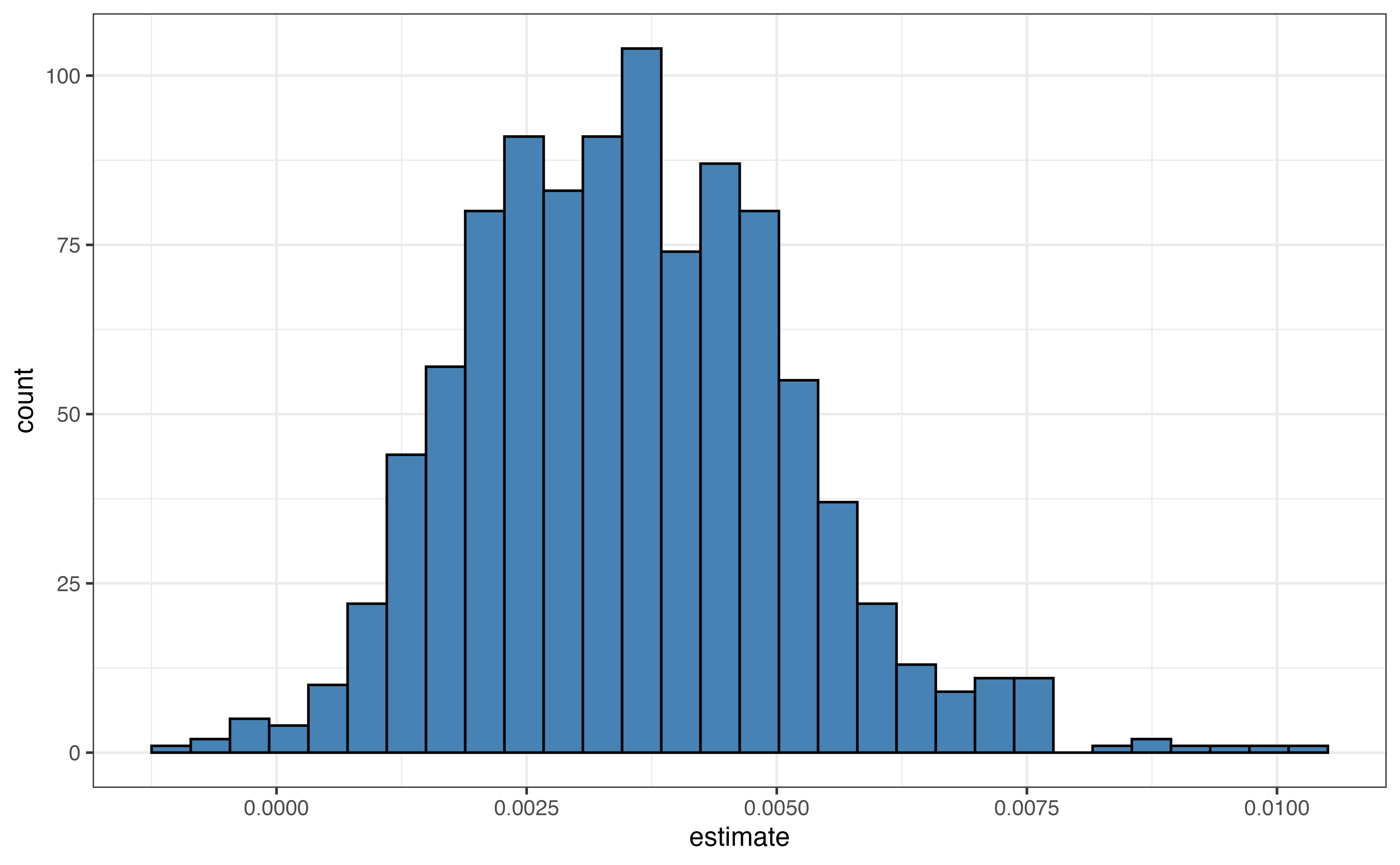

Finally, we can compute the lower and upper bounds for the confidence interval using the quantile function. Note that the code includes ungroup() , so that the data are not grouped by replicate.

boot_dist |> 
  ungroup() |>
  filter(term == "per_capita_expend") |>
  summarise(lb = quantile(estimate, 0.025),
            ub = quantile(estimate, 0.975))

# A tibble: 1 × 2
        lb      ub
     <dbl>   <dbl>
1 0.000735 0.00711

5.9.2 Permutation tests in R

The null distribution and p-value for the permutation test are computed using the infer package (Couch et al. 2021). Much of the code to generate the null distribution is similar to the code for the bootstrap distribution. Because permutation sampling is a random process, the code starts with set.seed() to ensure the results are reproducible.

1set.seed(12345)

2niter = 1000

3null_dist <- parks |>
4  specify(playgrounds ~ per_capita_expend) |>
5   hypothesize(null = "independence") |>
6  generate(reps = niter, type = "permute") |>
  fit()

1

Set a seed to make the results reproducible.

2

Define the number of bootstrap samples (iterations). Permutation sampling can be computing intensive when using large data sets and a large number of iterations. We recommend using a small number of iterations ( 10 - 100) when testing code, then increasing the iterations once the code is finalized.

3

Specify the data set and save the null distribution in the object null_dist.

4

Specify the response and predictor variable.

5

Specify the null hypothesis of “independence”, corresponding to no linear relationship between the response and predictor variables.

6

Specify the type of simulation (“permute”) and the number of iterations.

We can use ggplot to make a histogram of the null distribution.

null_dist |>
  filter(term == "per_capita_expend") |>
  ggplot(aes(x = estimate)) +
  geom_histogram()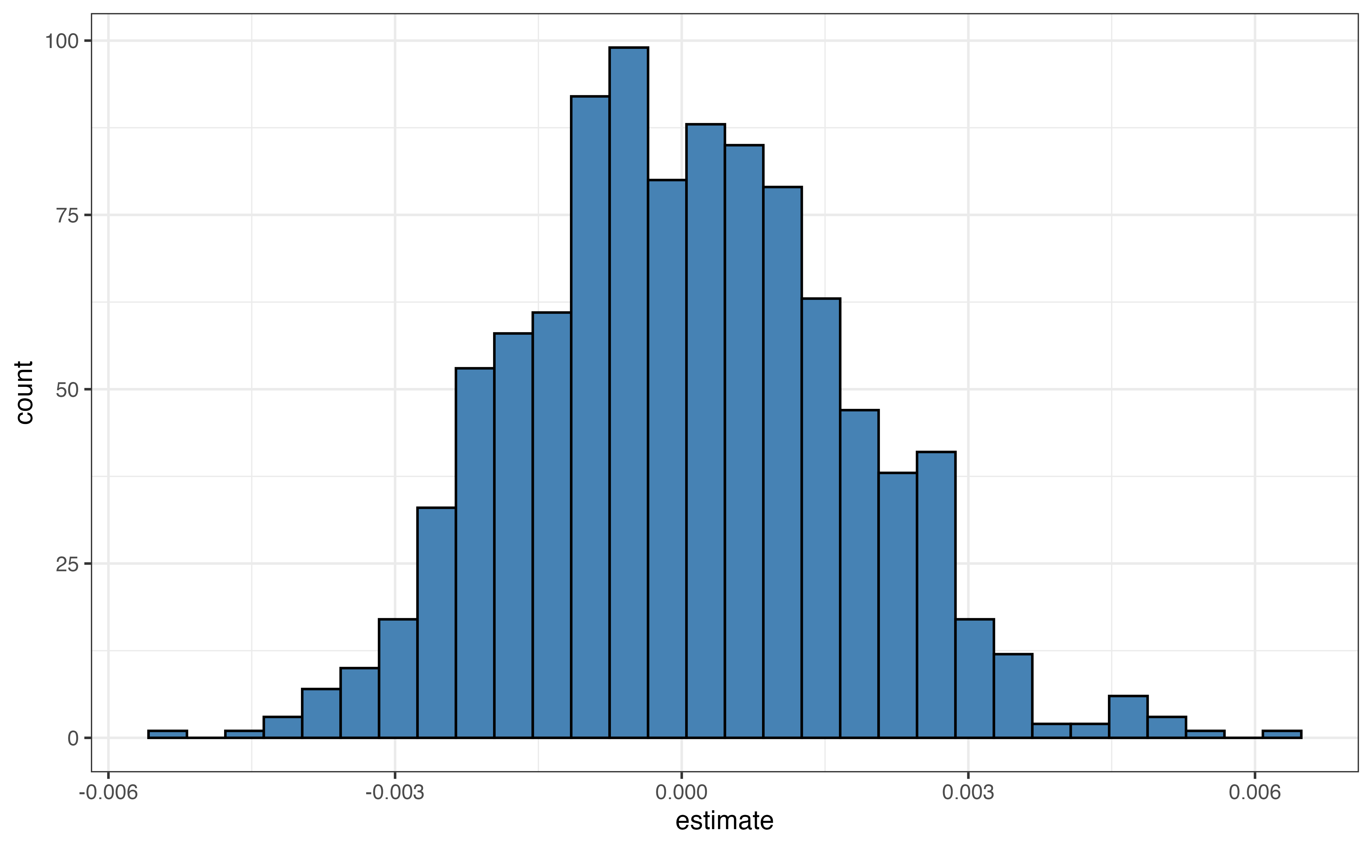

Finally, we compute the the p-value using the get_p_value().

# get estimated slope 
estimated_slope <- parks |>
  specify(playgrounds ~ per_capita_expend)  |> 
  fit()

# compute p-value 
get_p_value(null_dist, estimated_slope, direction = "both") |>
  filter(term == "per_capita_expend")

# A tibble: 1 × 2
  term              p_value
  <chr>               <dbl>
1 per_capita_expend   0.054

5.9.3 Theory-based inference in R

The output from lm() contains the statistics discussed in this section to conduct theory-based inference. The p-value in the output corresponds to the two-sided alternative hypothesis $H_a:{\beta }_1\ne 0$.

The confidence interval does not display by default, but can be added using the conf.int argument in the tidy function. The default confidence level is 95%; it can be adjusted using the conf.level argument in tidy().

parks_fit <- lm(playgrounds ~ per_capita_expend, data = parks)

tidy(parks_fit, conf.int = TRUE, conf.level= 0.95)

# A tibble: 2 × 7
  term              estimate std.error statistic  p.value conf.low conf.high
  <chr>                <dbl>     <dbl>     <dbl>    <dbl>    <dbl>     <dbl>
1 (Intercept)        2.42      0.214       11.3  3.11e-19 1.99       2.84   
2 per_capita_expend  0.00330   0.00160      2.06 4.24e- 2 0.000115   0.00648

In practice, we use the output from tidy() to get the confidence interval. To compute the confidence interval directly from the formula in Equation 5.11, we get ${\hat{\beta }}_1$ from the estimate column of the tidy() output and $S{E}_{{\hat{\beta }}_1}$ from the std.error column. The critical value is computed using the qt function. the first argument is the cumulative probability (the percentile associated with the upper bound of the interval), and the degrees of freedom go in the second argument. For example, the critical value for the 95% confidence interval for the parks data used in Equation 5.12 is

[1] 1.99

5.10 Summary

In this chapter we introduced two approaches for conducting statistical inference to draw conclusions about a population slope, simulation-based methods and theory-based methods. The standard error, test statistic, p-value and confidence interval we calculated using the mathematical models from the Central Limit Theorem align with what it seen from the output produced by statistical software in Table 5.2. Modern statistical software will produce these values for you, so in practice you will not typically derive these values “manually” as we did in this chapter. As the data scientist your role will be to interpret the output and use it to draw conclusions. It’s still valuable, however, to have an understanding of where these values come from in order to interpret and apply them accurately. As more software has embedded artificial intelligence features, understanding how the values are computed also helps us check if the software’s output makes sense given the data, analysis objective, and methods.

Which of these two methods is preferred to use in practice? In the next chapter, we will discuss the model assumptions from Section 5.3 and the conditions we use to evaluate whether the assumptions hold for our data. We will use these conditions in conjunction with other statistical and practical considerations to determine when we might prefer simulation-based methods or theory-based methods for inference.

Community, Data Science Learning. 2024. “Tidy Tuesday: A Weekly Social Data Project.” https://tidytues.day.

Couch, Simon P., Andrew P. Bray, Chester Ismay, Evgeni Chasnovski, Benjamin S. Baumer, and Mine Çetinkaya-Rundel. 2021. “Infer: An r Package for Tidyverse-Friendly Statistical Inference” 6: 3661. https://doi.org/10.21105/joss.03661.

The Trust for Public Land. 2021. “Parks and an Equitable Recovery.” Online.

---

1. Example: I think the relationship is positive. I predict that if the city spends more per resident, some of the funding is used for facilities like playgrounds.

2. Slope: For each additional dollar a city spends per resident, is expected to be 0.003 more playgrounds per 10,000 residents, on average.
   Intercept: We would not expect a city to invest $0 on services and facilities for its residents, so the interpretation of the intercept is not meaningful in practice.

3. We sample with replacement so that we get a new sample each time we bootstrap. If we sampled without replacement, we would always end up with a bootstrap sample is exactly the same as the original sample.

4. Each bootstrap sample is the same size as our current sample data. In this case, the sample data we’re analyzing has 97 observations.

5. There are 1000 values, the number of iterations, in the bootstrapped sampling distribution.

6. The points at the $5^{th}$ and ${95}^{th}$ percentiles make the bounds for the 95% confidence interval. The points at the $1^{st}$ and ${99}^{th}$ percentiles mark the lower and upper bounds for a 98% confidence interval.

7. The variability is approximately equal in both distributions. This is expected, because the distributions will have the same variability but different centers.

8. Given there is no linear relationship between spending per resident and playgrounds per 10,000 residents ( $H_0$ is true), the probability of observing a slope of 0.003 or more extreme in a random sample of 97 cities is 0.046.

9. It is possible we have made a Type I error, because we concluded to reject the null hypothesis.

10. Standard error is the term used for the standard deviation of a sampling distribution.

11. Note its similarities to the general equation for sample standard deviation, $s=\sqrt{\frac{\sum _{i=1}^n(y_i-\overline{y}{)}^2}{n-1}}$

12. Test statistics with small magnitude provide evidence in support of the null hypothesis, as they are close to the hypothesized value. Conversely test statistics with large magnitude provide evidence against the null hypothesis, as they are very far away from the hypothesized value.