4  Simple linear regression

Learning goals

• Use exploratory data analysis to assess whether a simple linear regression is an appropriate model to describe the relationship between two variables
• Estimate the slope and intercept for a simple linear regression model
• Interpret the slope and intercept in the context of the data
• Use the model to compute predictions and residuals
• Evaluate model performance using RMSE and $R^2$
• Conduct simple linear regression using R

4.1 Introduction: Movie ratings

Reviews from movie critics can be helpful when determining whether a movie is high quality and well-made; however, it can sometimes be challenging to determine whether regular audience members will like a movie based on critics reviews. We would like a way to better understand the relationship between what movie critics and regular movie goers think about a movie, and ultimately predict how an audience will rate a movie based on its score from movie critics.

To do so, we will analyze data that contains the critics scores and audience scores for 146 movies released in 2014 and 2015. The scores are for every movie released in these years that have “a rating on Rotten Tomatoes, a RT User rating, a Metacritic score, a Metacritic User score, an IMDb score, and at least 30 fan reviews on Fandango” (Albert Y. Kim, Ismay, and Chunn 2018a). The analysis in this chapter focuses on scores from Rotten Tomatoes, a website for information and ratings on movies and television shows. The data were originally analyzed in the article “Be Suspicious of Online Movie Ratings, Especially Fandango’s” (Hickey 2015) on the former data journalism website FiveThirtyEight. The data are available in movie_scores.csv. The data set was adapted from the fandago data frame in the fivethirtyeight R package (Albert Y. Kim, Ismay, and Chunn 2018b).

We will focus on two variables for this analysis:

• critics_score: The percentage of critics who have a favorable review of the movie. This is known as the “Tomatometer” score on the Rotten Tomatoes website. The possible values are 0 - 100.

• audience_score: The percentage of users (regular movie-goers) on Rotten Tomatoes who have a favorable review of the movie. The possible values are 0 - 100.

Our goal is to use simple linear regression to model the relationship between the critics score and audience score. We want to use the model to

• describe how the audience score is expected to change as the critics score changes.
• predict the audience score for a movie based on its critics score.

Recall from Section 1.1.1, the response variable is the outcome of interest, meaning the variable we are interested in predicting and understanding its variability. It is also known as the outcome or dependent variable and is represented as $Y$. The predictor variable(s) is the variable (or variables) used to understand variability in the response. It is also known as the explanatory or independent variable and represented as $X$. The observed values of the response and predictor are represented as $y_i$ and $x_i$, respectively.

What is the response variable for the movie scores analysis? What is the predictor variable?¹

4.2 Exploratory data analysis

Recall from Chapter 3 that we begin analysis with exploratory data analysis (EDA) to better understand the data, the distributions of key variables, and relationships in the data before fitting the regression model. The exploratory data analysis here focuses on the two variables that will be in the regression model, critics and audience. In practice, however, we may want to explore other variables in the data set (for example, year in this analysis) to provide additional context later on as we interpret results from the regression model. We begin with univariate EDA (Section 3.4), exploring one variable at a time, then we’ll conduct bivariate EDA (Section 3.5) to look at the relationship between the critics scores and audience scores.

4.2.1 Univariate EDA

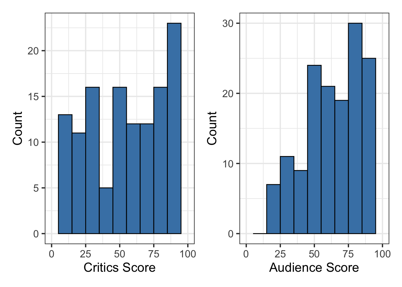
The univariate distributions of critics_score and audience_score are visualized in Figure 4.1 and summarized in Table 4.1.

(a) Critics score

(b) Adience score

Figure 4.1: Univariate distributions of critics_score and audience_score

Table 4.1: Summary statistics for critics_score and audience_score

Variable	Mean	SD	Min	Q1	Median (Q2)	Q3	Max	Missing
critics_score	60.8	30.2	5	31.2	63.5	89	100	0
audience_score	63.9	20.0	20	50.0	66.5	81	94	0

The distribution of critics_score is left-skewed, meaning the movies in the data set are generally more favorably reviewed by critics (more observations with higher critics scores). Given the apparent skewness, the center is best described by the median score of 63.5 points. The interquartile range (IQR), the spread of the middle 50% of the distribution, is 57.8 points $(Q_3-Q_1=89-31.2)$, so there is a lot of variability in the critics scores for the movies in the data. There are no apparent outliers, but we observe from the raw data that there are two notable observations of movies that have perfect critics scores of 100. There are no missing values of critics score.

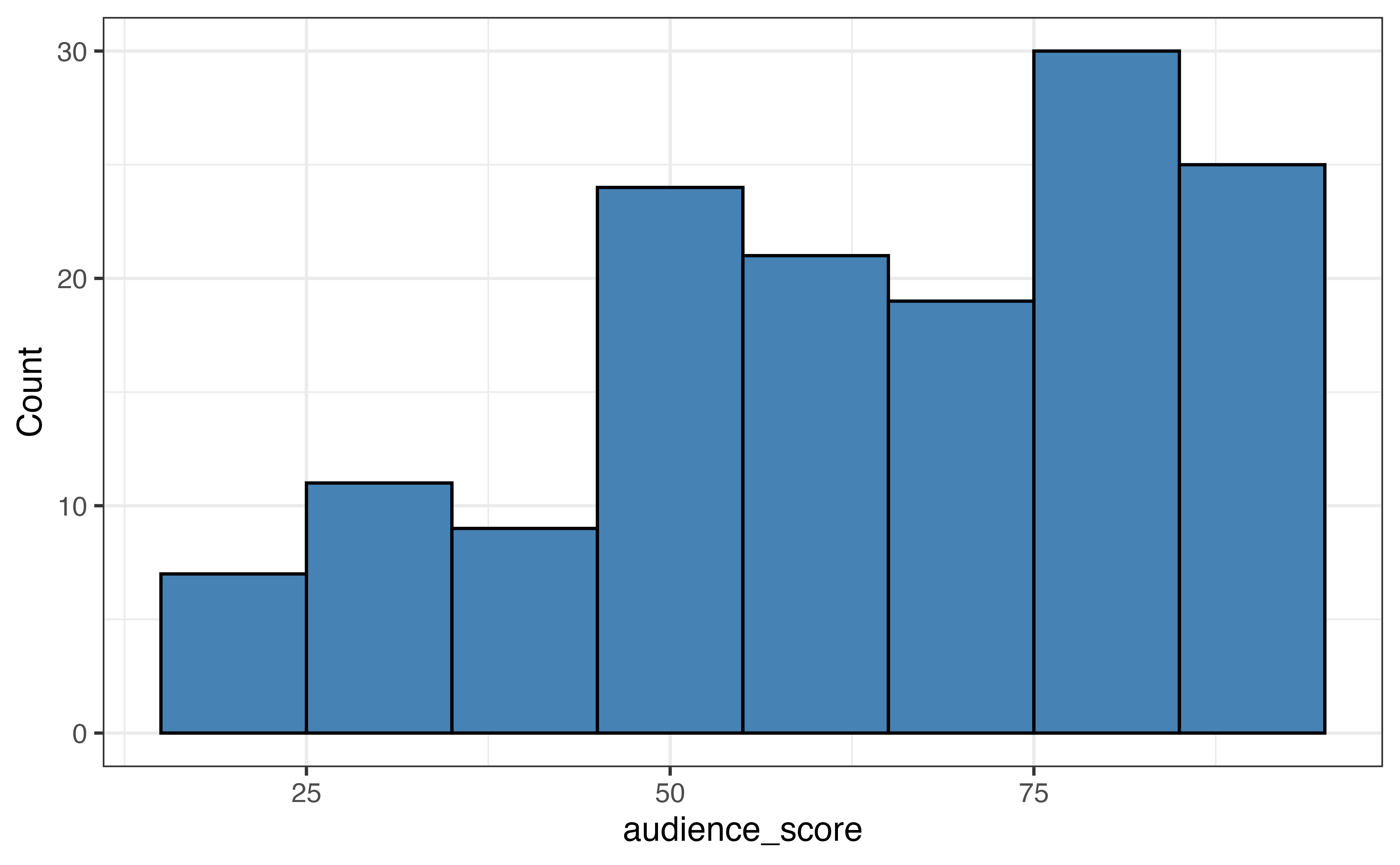
Use the histogram in Figure 4.1 (b) and summary statistics in Table 4.1 to describe the distribution of the response variable audience_score.²

4.2.2 Bivariate EDA

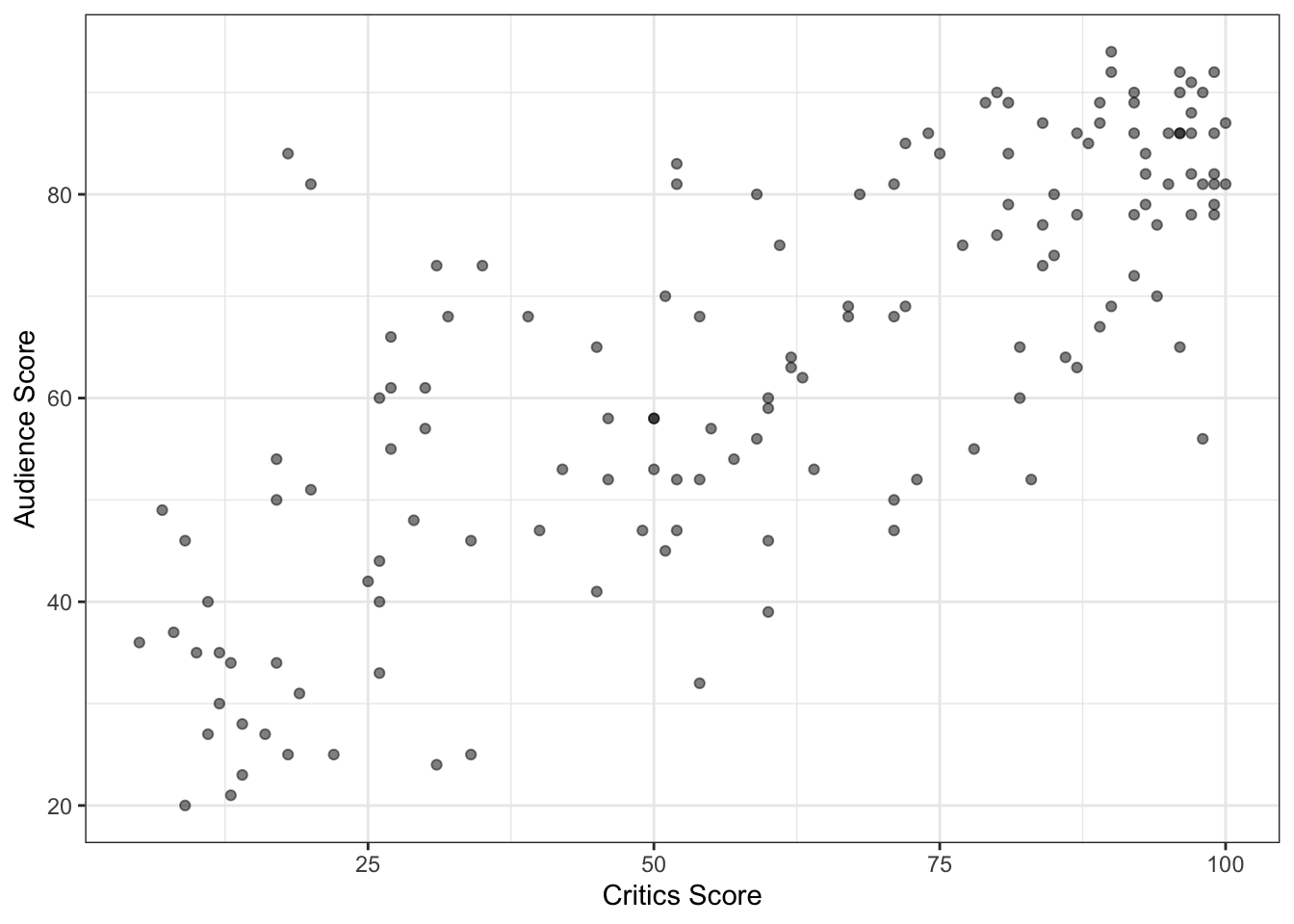
Now let’s look at the relationship between critics_score and audience_score. From Section 3.5.1, we use visualizations and summary statistics to examine the relationship between two quantitative variables. A scatterplot of the the audience score versus critics score is shown in Figure 4.2. The predictor variable is on the $x$-axis (horizontal axis), and the response variable is on the $y$-axis (vertical axis).

Figure 4.2: Scatterplot of critics_score and audience_score

There is a positive, linear relationship between the critics scores and audience scores for the movies in our data. The correlation between these two variables is 0.78, indicating the relationship is strong. Therefore, we can generally expect the audience score to be higher for movies with higher critics scores. There are no apparent outliers, but there does appear to be more variability in the audience score for movies with lower critics scores than for those with higher critics scores.

4.3 Linear regression

In Section 4.2, we used visualizations and summary statistics to describe the relationship between two variables. The exploratory data analysis, however, does not tell us what the audience score is predicted to be for a given value of the critics score or how much the audience score is expected to change as the critics score changes. Therefore, we will fit a linear regression model to quantify the relationship between the two variables. Recall the general form of the linear regression model in Equation 1.3. More specifically, when we have one predictor variable, we will fit a model of the form

$$\begin{array}{}\text{(4.1)}& Y={\beta }_0+{\beta }_{1}X+ϵϵ\sim N(0,{\sigma }_{ϵ}^2)\end{array}$$

Equation 4.1, called a simple linear regression (SLR) model, is the equation to model the relationship between one quantitative response variable and one predictor variable. For now we will focus on models with one quantitative predictor variable. In later chapters, we will introduce models with two or more predictors (Chapter 7), categorical predictors (Section 7.4.2), and models with a categorical response variable (Chapter 11).

We are generally interested in using regression models for two types of tasks:

• Prediction: Finding the expected value of the response variable for given values of the predictor variable(s).
• Inference: Drawing conclusions about the relationship between the response and predictor variables.

Suppose we fit a simple linear regression line to summarize the relationship between critics_score and audience_scores for movies.

• What is an example of a prediction question that can be answered using a simple linear regression model?
• What is an example of an inference question that can be answered using a simple linear regression model?³

4.3.1 Statistical (theoretical) model

We expand on the concepts introduced in Section 1.1.1 for the simple linear regression model. Suppose there is a response variable $Y$ and a predictor variable $X$. The values of the response variable $Y$ can be generated in the following way:

$$\begin{array}{}\text{(4.2)}& Y=\text{Model}+\text{Error}\end{array}$$

More specifically, we define the model as a function of the predictor $X$, $\text{Model}=f(X)$, and error $ϵ$, such that

$$\begin{array}{}\text{(4.3)}& Y=f(X)+ϵ\end{array}$$

The function $f(X)$ that describes the relationship between the response and predictor variables is the regression model. This is the model we will fit in later sections using equations and software. The error, $ϵ$, is how much the actual value of the response $Y$ deviates from the value produced by the regression model, $f(X)$. There is some randomness in $ϵ$, because not all observations with the same value of $X$ have the same value of $Y$. For example, not all movies with a critics score of 70 have the same audience score.

Equation 4.3 is the general form of the equation to generate values of $Y$ given values of $X$. In the context of simple linear regression, the function $f(X)$ in Equation 4.3 is

$$\begin{array}{}\text{(4.4)}& f(X)={\mu }_{Y|X}={\beta }_0+{\beta }_{1}X\end{array}$$

where ${\mu }_{Y|X}$ is the mean value of $Y$ at a particular value of $X$, and ${\beta }_0$ and ${\beta }_1$ are the model coefficients. The error terms $ϵ$ from Equation 4.3 are normally distributed with a mean of 0 and variance ${\sigma }_{ϵ}^2$, represented as $N(0,{\sigma }_{ϵ}^2)$ (more on this in Section 5.3. The specification of the simple linear regression model written in terms of individual observations $(x_i,y_i)$ is

$$\begin{array}{}\text{(4.5)}& y_i={\beta }_0+{\beta }_1{x}_i+{ϵ}_i{ϵ}_i\sim N(0,{\sigma }_{ϵ}^2)\end{array}$$

such that $y_i$ is the response for the $i^{th}$ observation, $x_i$ is he predictor for the $i^{th}$ observation, and ${ϵ}_i$ is the error for the $i^{th}$ observation. Equation 4.5 is the statistical model, also called the data-generating model or population-level model. It is the theoretical form of the model that describes exactly how to generate the values of the response $Y$ given values of the predictor in the population. The model coefficients are the intercept ${\beta }_0$ and the slope ${\beta }_1$. The${\sigma }_{ϵ}^2$ is called the standard error. In practice we don’t know the exact values of ${\beta }_0$, ${\beta }_1$, and ${\sigma }_{ϵ}^2$, so our goal is to use sample data to estimate these values. We will focus on the coefficients ${\beta }_0$ and ${\beta }_1$ in this chapter. We discuss estimating ${\sigma }_{ϵ}^2$ in Section 5.8.2.

In simple linear regression, we use sample data to estimate a model to understand trends in the population.

What is the population in the movie scores analysis? What is the sample?⁴ Recall the definition of population and sample in Section 1.1.

4.3.2 Evaluating whether SLR is appropriate

Before doing any more calculations, we need to determine if the simple linear regression model is a reasonable choice to summarize the relationship between the response variable and predictor variable based on what we know about the data and what we’ve observed from the exploratory data analysis. Determining this early on can help prevent going in a wrong analysis direction if a linear regression model is obviously not a good choice for the data.

We can ask the following questions to evaluate whether simple linear regression is appropriate:

• Will a linear regression model be practically useful? Does quantifying and interpreting the relationship between the variables make sense in this scenario?
• Is the shape of the relationship reasonably linear?
• Do the observations in the data represent the population of interest, or are there biases in the data that could limit conclusions drawn from the analysis?

Mathematical equations or statistical software can be used to fit a linear regression model between any two quantitative variables. Therefore it is upon the judgment of the data scientist to determine if it is reasonable to proceed with a linear regression model or if doing so might result in misleading conclusions about the data. If the answer is “no” to any of the questions above, consider if a different analysis technique is better for the data, or proceed with caution if using regression. If we proceed with regression, be transparent about some of the limitations of the conclusions.

From Section 4.1, the goal of this analysis is understand the relationship between the critics scores and audience score for movies on Rotten Tomatoes. Therefore, there is a practical use for fitting the regression model. We observed from Figure 4.2 that the relationship between the two variables is approximately linear, so it could reasonably be summarized a model of the form of Equation 4.5. Lastly, the data set includes all movies in 2014 and 2015 that has a sufficient number of ratings on popular movie ratings websites, so we can reasonably conclude the sample is representative of the population of movies on Rotten Tomatoes. Therefore, we are comfortable drawing conclusions about the population based on the analysis of our sample data.

The form of the simple linear regression model for the movie scores data is

$$\begin{array}{}\text{(4.6)}& \text{audience\_score}={\beta }_0+{\beta }_1\text{critics\_score}+ϵ,ϵ\sim N(0,{\sigma }_{ϵ}^2)\end{array}$$

Now that we have the form of the model, let’s discuss how to estimate and interpret the model coefficients, the slope ${\beta }_1$ and the intercept ${\beta }_0$. We will estimate ${\sigma }_{ϵ}^2$ in Chapter 5.

4.4 Estimating the model coefficients

Ideally, we would have data from the entire population of movies rated on Rotten Tomatoes in order to calculate the exact values for ${\beta }_0$ and ${\beta }_1$. In reality we don’t have access to the data from the entire population, but we can use the sample to obtain the estimated regression equation in Equation 4.7

$$\begin{array}{}\text{(4.7)}& {\hat{y}}_i={\hat{\beta }}_0+{\hat{\beta }}_1{x}_i\end{array}$$

where ${\hat{\beta }}_0$ is the estimated intercept, ${\hat{\beta }}_1$ is the estimated slope, and ${\hat{y}}_i$ is the predicted (estimated) response.

Specifically for the movie scores analysis, the estimated regression equation is

$$\begin{array}{}\text{(4.8)}& {\widehat{\text{audience\_score}}}_i=32.316+0.519{\text{critics\_score}}_i\end{array}$$

In this equation 32.316 is ${\hat{\beta }}_0$, the estimated value for the intercept, 0.519 is ${\hat{\beta }}_1$, the estimated value for the slope ${\beta }_1$, and ${\widehat{\text{audience\_score}}}_i$ is the expected audience score when the critics score is equal to ${\text{critics\_score}}_i$. Notice that Equation 4.7 and Equation 4.8 do not have have error term, $ϵ$. The output from the regression equation is $\widehat{f(X)}={\hat{\mu }}_{Y|X}$, the expected mean value of the response given a value of the predictor. Therefore, when we discuss the values of the response estimated using simple linear regression, what we are really talking about is what the value of the response variable is expected to be, on average, for a given value of the predictor variable.

From Figure 4.2, we know that the value of the response is not necessarily the same for all observations with the same value of the predictor. For example, we wouldn’t expect (nor do we observe) the same audience score for every movie with a critics score of 70. We know there are other factors other than the critics score that are related to how an audience reacts to a movie. Our analysis, however, only takes into account the critics score, so we do not capture these additional factors in our regression equation Equation 4.8. This is where the error terms come back in.

Once we computed estimates ${\hat{\beta }}_0$ and ${\hat{\beta }}_1$ for the regression equation, we can calculate how far the predicted values of the response produced by the regression equation differ from the actual values of the response variable observed in the data. This difference is called the residual, denoted $e_i$.

Equation 4.9 shows the equation of the residual for the $i^{th}$ observation.

$$\begin{array}{}\text{(4.9)}& e_i={\text{observed}}_i-{\text{predicted}}_i=y_i-{\hat{y}}_i\end{array}$$

In the case of the movie scores data, the residual is the difference between the actual audience score and the audience score predicted by Equation 4.8. For example, the 2015 movie Avengers: Age of Ultron received a critics score of $y_i=74$. Therefore, using Equation 4.8, the estimated (predicted) audience score is.

$${\hat{y}}_i=32.316+0.519\times 74=70.722.$$

The observed audience score is 86, so the residual is

$$e_i=y_i-{\hat{y}}_i=86-70.722=15.278$$

Would you rather see a movie that has a positive or negative residual? Explain your response.⁵

4.4.1 Least squares regression

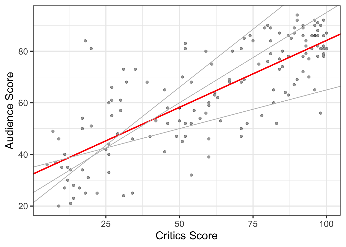
There are many possible regression lines (infinitely many, in fact) that we could use to summarize the relationship between critics_score and audience_scores. We see some fo the potential lines represented in Figure 4.3. So how did we determine the line that “best” fits the data is the one described by Equation 4.8? We’ll use the residuals to help us answer this question.

Figure 4.3: Potential regression lines for the relationship between critics_score and audience_score

The residuals, represented by the vertical dotted lines in Figure 4.4, are a measure of the “error”, the difference between the observed value of the response and the value predicted from a regression model. The line that “best” fits the data is the one that generally results in the smallest overall error. One way to find the line with the smallest overall error is to add up all the residuals for each possible line in Figure 4.3 and choose the one that has the smallest sum. Notice, however, that for lines that seem to closely align with the trend of the data, there is approximately equal distribution of points above and below the line. Thus as we’re trying to compare lines that pretty closely fit the data, we’d expect the residuals to add up to a value very close to zero. This would make it difficult, then, to determine a best fit line.

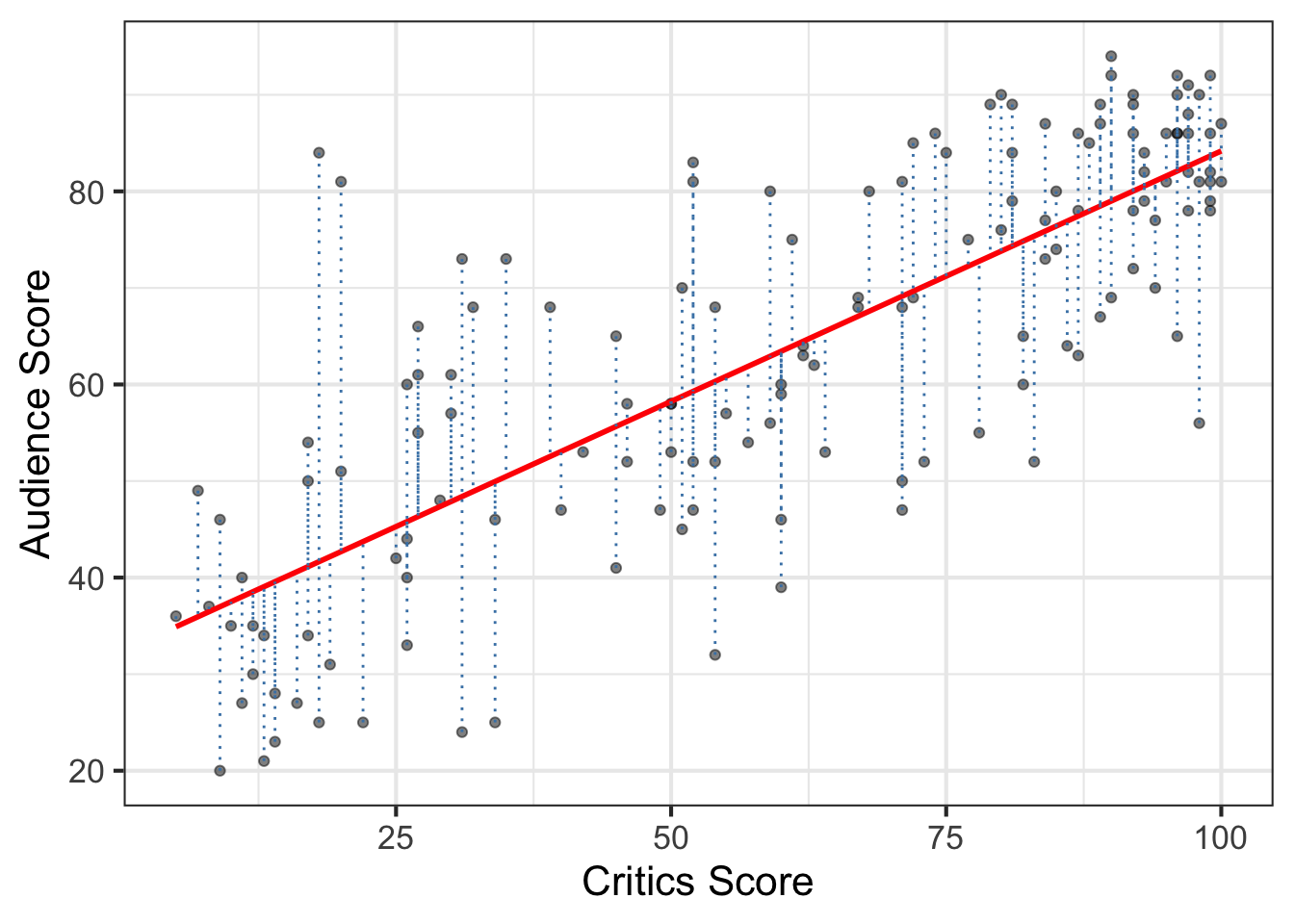
Figure 4.4: Regression line of the relationship between critics_score and audience_score with residuals

Instead of using the sum of the residuals, we will instead consider the sum of the squared residuals in Equation 4.10

$$\begin{array}{}\text{(4.10)}& \sum _{i=1}^n{e}_i^2=e_1^2+e_2^2+\cdots +e_n^2\end{array}$$

where $n$ is the number of observations in the data. The line that “best” fits the data, then, is the line that minimizes Equation 4.10. This is called the least squares regression model.

Let’s expand Equation 4.10. Recall that $e_i$, the residual of the $i^{th}$ observation, is $y_i-{\hat{y}}_i$ where ${\hat{y}}_i$ is the estimated response. Then,

$$\begin{array}{}\text{(4.11)}& \begin{array}{rl}{e}_i& =y_i-{\hat{y}}_i\\ & =y_i-({\hat{\beta }}_0+{\hat{\beta }}_1{x}_i)\end{array}\end{array}$$

Thus, putting Equation 4.11 into Equation 4.10, we have

$$\begin{array}{}\text{(4.12)}& \begin{array}{rl}\sum _{i=1}^n{e}_i^2& =e_1^2+e_2^2+\cdots +e_n^2\\ & =[y_1-({\hat{\beta }}_0+{\hat{\beta }}_1{x}_1){]}^2+[y_2-({\hat{\beta }}_0+{\hat{\beta }}_1{x}_2){]}^2+& \\ & \cdots +[y_n-({\hat{\beta }}_0+{\hat{\beta }}_1{x}_n){]}^2\end{array}\end{array}$$

Using calculus, the ${\hat{\beta }}_0$ and ${\hat{\beta }}_1$ that minimize Equation 4.12 are

$$\begin{array}{}\text{(4.13)}& {\hat{\beta }}_1=r\frac{s_Y}{s_X}{\hat{\beta }}_0=\overline{y}-{\hat{\beta }}_1\overline{x}\end{array}$$

where $\overline{x}$ and $\overline{y}$ are the mean values of the predictor and response variables, respectively, $s_X$ and $s_Y$ are the standard deviations of the predictor and response variables, respectively, and $r$ is the correlation between the response and predictor variables. See Appendix A.1 for the full details of the derivation from Equation 4.12 to Equation 4.13.

Equation 4.14 show the calculations of slope and intercept for the movie scores model based on the summary statistics in Table 4.1. Note that the small differences in the values compared to Equation 4.8 are due to rounding (versus coefficients computed by software).

$$\begin{array}{}\text{(4.14)}& \begin{array}{rl}{\hat{\beta }}_1& =0.78\times \frac{20.0}{30.2}=0.517\\ {\hat{\beta }}_0& =63.9-0.517\times 60.8=32.467\end{array}\end{array}$$

Below are a few properties of least-squares regression models.

• The regression line goes through the center of mass point, the coordinates corresponding to average $X$ and average $Y$: ${\hat{\beta }}_0=\overline{y}-{\hat{\beta }}_1\overline{x}$

• The slope has the same sign as the correlation coefficient: ${\hat{\beta }}_1=r\frac{s_Y}{s_X}$

• The sum of the residuals is zero: $\sum _{i=1}^n{e}_i=0$

• The residuals and values of the predictor are uncorrelated

4.5 Interpreting the model coefficients

The slope ${\hat{\beta }}_1$ is the estimated change in the response for each unit increase in the predictor variable. What do we mean by “estimated change”? Recall that the output from the regression equation is ${\mu }_{Y|X}$ the estimated mean of the response $Y$ for a given value of the predictor $X$. Thus, the slope or the “steepness” of the regression line, is a measure of how much the response variable is expected to change, on average, for each unit increase of the predictor.

It is good practice to write the interpretation of the slope in the context of the data, so that it can be more easily understood by others reading the analysis results. “In the context of the data” means that the interpretation includes

• meaningful descriptions of the variables, if the variable names would be unclear to an outside reader
• units for each variable
• an indication of the population for which the model applies.

The slope in Equation 4.8 of 0.519 is interpreted as the following:

For each additional point in the critics score, the audience score for movies on Rotten Tomatoes is expected to increase by 0.519 points, on average.

The intercept is the estimated value of the response variable when the predictor variable equals zero $(x_i=0)$. On a scatterplot of the response and predictor variable, this is the point where the regression line crosses the $y$-axis. Similar to the slope, the “estimated value” is more specifically the estimated mean value of the response variable when the predictor equals 0 ( ${\hat{\mu }}_{Y|X=0})$.

The intercept in Equation 4.8 of 32.316 is interpreted as the following:

The expected audience score for movies on Rotten Tomatoes with a critics score of 0 is 32.316 points.

We always need to estimate the intercept in ?eq-regressio to get the line that best fit using least squares regression. The intercept, however, does not always have a meaningful interpretation. We ask the following questions to determine if the intercept has a meaningful interpretation:

1. Is it plausible for the predictor variable to take values at or near zero?

2. Are there observations in the data with values of the predictor at or near zero?

If the answer to either question is no, then it is not meaningful, and potentially misleading, to interpret the intercept.

Is the interpretation of the intercept in Equation 4.8 meaningful? Briefly explain.⁶

Avoid using causal language and making declarative statements (e.g., “The audience score for a movie with a critics score of 0 points will be 32.316 points.”) when interpreting the slope and intercept. Remember the slope and intercept are estimates describing what is expectedin the relationship between the response and predictor to be based on the sample data and linear regression model. They do not tell us exactly what will happen in the data.

There is an area of statistics called causal inference about model that can be used to make causal statements from observational (non-experimental) data. See Section 13.4 for a brief introduction to causal inference.

4.6 Prediction

One of the primary purposes of a regression model is to use for prediction. When a regression model is used for prediction, the estimated value of the response variable is computed based on a given value of the predictor. We’ve seen this in earlier sections when calculating the residuals. Let’s take a look at the model predictions for two movies released in 2023.

The movie Barbie was released in theaters on July 21, 2023. This movie was widely praised by critics, and it has a critics score of 88 at the time the data were obtained. Based on Equation 4.8, the predicted audience score is

$$\begin{array}{rl}\widehat{\text{audience\_scores}}& =32.316+0.519\times 88\\ & =\mathbf{\text{77.988}}\end{array}$$

From the snapshot of the Barbie Rotten Tomatoes page (Figure 4.5), we see the actual audience score is 83⁷. Therefore, the model under predicted the audience score by about 5 points (83 - 77.988). Perhaps this isn’t surprising given this film’s massive box office success!

Figure 4.5: Source: https://www.rottentomatoes.com/m/barbie (accessed August 29, 2023)

The movie Asteroid City was released in theaters on June 23, 2023. The critics score for this movie was 75⁸.

• What is the predicted audience score?

• The actual audience score is 62. Did the model over or under predict? What is the residual? ⁹

The regression model is most reliable when predicting the response for values of the predictor within the range of the sample data used to fit the regression model. Using the model to predict for values far outside this range is called extrapolation. The sample data provide information about the relationship between the response and predictor variables for values within the range of the predictor in the data. We can not safely assume that the linear relationship quantified by our model is the same for values of the predictor far outside of this range. Therefore, extrapolation often results in unreliable predictions that could be misleading if the linear relationship does not hold outside the range of the sample data.

Only use the regression model to compute predictions for values of the predictor that are within (or very close) to the range of values in the sample data used to fit the model. Extrapolation, using a model to compute predictions for value so the predictor far outside the range in the data, can result in unreliable predictions.

4.7 Model evaluation

We have shown how a simple linear regression model can be used to describe the relationship between a response and predictor variable and to predict new values of the response. Now we will look at two statistics that will help us evaluate how well the model fits the data and how well it explains variability in the response.

4.7.1 Root Mean Square Error

The Root Mean Square Error (RMSE), shown in Equation 4.15, is a measure of the average difference between the observed and predicted values of the response variable.

$$\begin{array}{}\text{(4.15)}& RMSE=\sqrt{\frac{\sum _{i=1}^n{e}_i^2}{n}}=\sqrt{\frac{\sum _{i=1}^n(y_i-{\hat{y}}_i{)}^2}{n}}\end{array}$$

This measure is especially useful if prediction is the primary modeling objective. The RMSE takes values from 0 to $\mathrm{\infty }$ (infinity) and has the same units as the response variable.

Do higher or lower values of RMSE indicate a better model fit?¹⁰

There is no universal threshold of RMSE to determine whether the model is a good fit. In fact, the RMSE is often most useful when comparing the performance of multiple models. Take the following into account when using RMSE to evaluate model fit.

1. What is the range $(\text{max}-\text{min})$ of the response variable in the data? How does the RMSE compare to the range? For example, $RMSE=10$ indicates very good model performance if the response variable ranges from 10000 to 20000, but very poor model performance if the response variable ranges from 0 to 20.
2. What is a reasonable error threshold based on the subject matter and analysis objectives? We may be willing to use a model with higher RMSE for a low-stakes analysis objective (for example, the model is used to inform the choices of movie-goers) than a high-stakes objective (the model is used to inform how a movie studio’s multi-million dollar marketing budget will be allocated).

The RMSE for the movie scores model is 12.452. The range for the audience score is -. What is your evaluation of the model fit based on RMSE? Explain your response.¹¹

4.7.2 Analysis of variance and $R^2$

The coefficient of determination, $R^2$, the percentage of variability in the response variable that is explained by the predictor variable. In terms of the movie scores data, it is the percentage of variability in the audience score that is accounted for by changes in the critics score. Before talking more about how $R^2$ is used for model evaluation, let’s discuss how this percentage is calculated.

There is variability in the response variable, as we see in the exploratory data analysis in Figure 4.1 and Table 4.1. Analysis of Variance (ANOVA), shown in Equation 4.16, is the process of partitioning the various sources of variability.

$$\begin{array}{}\text{(4.16)}& \text{Total variability}=\text{Explained variability}+\text{Unexplained variability}\end{array}$$

From Equation 4.16, the variability in the response variable is from two sources:

1. Explained variability (Model): This is the variability in the response variable that can be explained by the model. In the case of simple linear regression, it is the variability in the response variable that can be explained by the predictor variable. In the movie scores analysis, this is the variability in audience_score that is explained by the critics_score.

2. Unexplained variability (Residuals): This is the variability in the response variable that is left unexplained after the model is fit. This can be understood by assessing the variability in the residuals. In the movie scores analysis, this is the variability due to the factors other than critics score.

The variability in the response variable and the contribution from each source is quantified using sum of squares. In general, the sum of squares (SS) is a measure of how far the observations are from a given point, for example the mean. Using sum of squares, we can quantify the components of Equation 4.16.

Let $SST$ = Sum of Squares Total, $SSM$ = Sum of Squares Model, and $SSR$ = Sum of Squares Residuals. Then,

$$\begin{array}{}\text{(4.17)}& \begin{array}{rl}SST& =SSM+SSR\\ \sum _{i=1}^n(y_i-\overline{y}{)}^2& =\sum _{i=1}^n({\hat{y}}_i-\overline{y}{)}^2+\sum _{i=1}^n(y_i-{\hat{y}}_i{)}^2\end{array}\end{array}$$

Sum of Squares Total (SST) $=\sum _{i=1}^n(y_i-\overline{y}{)}^2$, is the total variability, an overall measure of how far the observed values of the response variable are from the mean value of the response $\overline{y}$. The formula for SST may look familiar, as it is $(n-1)s_y^2$ , which equals$(n-1)$ times the variance of $y$. SST can be partitioned into two pieces, Sum of Squares Model (SSM) and Sum of Squares Residuals (SSR).

Sum of Squares Model (SSM) $=\sum _{i=1}^n({\hat{y}}_i-\overline{y}{)}^2$, is the explained variability, an overall measure of how much the predicted value of the response variable (the expected mean value of the response given the predictor) differs from the overall mean value of the response. This indicates how much the observed response’s deviation from the mean is accounted for by knowing the value of the predictor.

Lastly, the Sum of Squares Residual (SSR) $=\sum _{i=1}^n(y_i-{\hat{y}}_i{)}^2$, is the unexplained variability, an overall measure of how much the observed values of the response differ from the predicted values. This is the same sum of squared residuals used to estimate the least-squares regression model in Section 4.4.1.

We use the sum of squares to calculate the coefficient of determination $R^2$

$$\begin{array}{}\text{(4.18)}& R^2=\frac{SSM}{SST}=1-\frac{SSR}{SST}\end{array}$$

Equation 10.1, shows that $R^2$ is a the proportion of variability in the response (SST) that is explained by the model (SSM). Note that $R^2$ is calculated as proportion between 0 and 1, but is reported as a percentage between 0% and 100%.

The $R^2$ for the model in Equation 4.8 is 0.611. It is interpreted as the following:

About 61.1% of the variability in the audience score for movies on Rotten Tomatoes can be explained by the model (critics score).

Do higher or lower values of $R^2$ indicate a better model fit?¹²

Similar to RMSE, there is no universal threshold for what makes a “good” $R^2$ value. When using $R^2$ to determine if the model is a good fit, take into account what might be a reasonable to expect given the subject matter.

4.8 Simple linear regression in R

4.8.1 Fitting the least-squares model

We fit linear regression models using the lm function, which is part of the stats package (2024) built into R. We then use the tidy function from the broom package (Robinson, Hayes, and Couch 2023) to display the results in a tidy data format (Section 2.3.1). The code to find the linear regression model using the movie_scores data with audience_score as the response and critics_score as the predictor (Equation 4.8) is below.

lm(audience_score ~ critics_score, data = movie_scores)

Call:
lm(formula = audience_score ~ critics_score, data = movie_scores)

Coefficients:
  (Intercept)  critics_score  
       32.316          0.519  

Next, we want to display the model results in a tidy format. We build upon the code above by saving the model in an object called movie_fit and displaying the object. We will also use movie_fit to calculate predictions.

movie_fit <- lm(audience_score ~ critics_score, data = movie_scores) 

tidy(movie_fit) 

# A tibble: 2 × 5
  term          estimate std.error statistic  p.value
  <chr>            <dbl>     <dbl>     <dbl>    <dbl>
1 (Intercept)     32.3      2.34        13.8 4.03e-28
2 critics_score    0.519    0.0345      15.0 2.70e-31

Notice the resulting the model is the same as Equation 4.8, which we calculated based on Equation 4.13. We will discuss the other columns in the output in Chapter 5.

We can also use kable() from the knitr package (Xie 2024) to display the tidy results in an neatly formatted table and control the number of digits in the output.

tidy(movie_fit) |>
  kable(digits = 3)

term	estimate	std.error	statistic	p.value
(Intercept)	32.316	2.343	13.8	0
critics_score	0.519	0.035	15.0	0

4.8.2 Prediction

Below is the code to predict the audience score for Barbie as shown earlier in the section. We create a tibble that contains the critics score for Barbie, then use predict() and the model object to compute the prediction.

barbie_movie <- tibble(critics_score = 88) 
predict(movie_fit, barbie_movie)

 1 
78 

We can also produce predictions for multiple movies by putting multiple values of the predictor in the tibble. In the code below we produce predictions for Barbie and Asteroid City. We begin by storing the critics scores for both movies in a tibble. Then we use predict(), as before.

new_movies <- tibble(critics_score = c(88, 75)) 
predict(movie_fit, new_movies) 

   1    2 
78.0 71.2 

4.8.3 $R^2$ and RMSE

The glance() function in the broom package produces model summary statistics, including $R^2$.

glance(movie_fit)

# A tibble: 1 × 12
  r.squared adj.r.squared sigma statistic  p.value    df logLik   AIC   BIC
      <dbl>         <dbl> <dbl>     <dbl>    <dbl> <dbl>  <dbl> <dbl> <dbl>
1     0.611         0.608  12.5      226. 2.70e-31     1  -575. 1157. 1166.
# ℹ 3 more variables: deviance <dbl>, df.residual <int>, nobs <int>

The code below will only return $R^2$ from the output of glance().

glance(movie_fit)$r.squared

[1] 0.611

RMSE is computed using the rmse() function from the yardstick package (Kuhn, Vaughan, and Hvitfeldt 2025). First, we use augment() from the broom package to compute the predicted value for each observation in the data set. These values are stored if the column .fitted. We may notice that many other columns are produced by augment() as well; these are discussed in Chapter 6. We input the augmented data into rmse().

movies_augment <- augment(movie_fit) 

rmse(movies_augment, truth = audience_score, estimate = .fitted) 

# A tibble: 1 × 3
  .metric .estimator .estimate
  <chr>   <chr>          <dbl>
1 rmse    standard        12.5

4.9 Summary

In this chapter, we introduced simple linear regression. We showed how to use exploratory data analysis to evaluate whether linear regression is appropriate to model the relationship between two variables. Next, we computed the slope and intercept (the model coefficients) and interpreted these values in in the context of the data. We used the model to compute predictions and evaluated the model performance using $R^2$ and RMSE. We finished the chapter by conducting simple linear regression in R.

This chapter has helped set the foundation for all the regression methods presented throughout the remainder of the text. In Chapter 5, we’ll use the simple linear regression model to draw conclusions about the relationship between the response and predictor variables.

Hickey, Walt. 2015. “Be Suspicious of Online Movie Ratings, Especially Fandango’s.” FiveThirtyEight, Available at: Http://Fivethirtyeight. Com/Features/Fandango-Movies-Ratings.

Kim, Albert Y., Chester Ismay, and Jennifer Chunn. 2018a. “The Fivethirtyeight r Package: ’Tame Data’ Principles for Introductory Statistics and Data Science Courses” 11. https://escholarship.org/uc/item/0rx1231m.

Kim, Albert Y, Chester Ismay, and Jennifer Chunn. 2018b. “The Fivethirtyeight r Package:‘tame Data’principles for Introductory Statistics and Data Science Courses.” Technology Innovations in Statistics Education 11 (1).

Kuhn, Max, Davis Vaughan, and Emil Hvitfeldt. 2025. “Yardstick: Tidy Characterizations of Model Performance.” https://doi.org/10.32614/CRAN.package.yardstick.

R Core Team. 2024. “R: A Language and Environment for Statistical Computing.” https://www.R-project.org/.

Robinson, David, Alex Hayes, and Simon Couch. 2023. “Broom: Convert Statistical Objects into Tidy Tibbles.” https://CRAN.R-project.org/package=broom.

Xie, Yihui. 2024. “Knitr: A General-Purpose Package for Dynamic Report Generation in r.” https://yihui.org/knitr/.

---

1. The response variable is audience, the audience score. The predictor variable is critics, the critics score.

2. The distribution of audience_score is unimodal and left-skewed. The median score is 66.5 and the IQR is 31 (81 - 50). We note that the center is higher and there is less variability in the middle 50% of the distribution compared to critics_score .

3. Example prediction question: What do we expect the audience score to be for movies with a critics score of 75?
   Example inference question Is the critics score a useful predictor of the audience score?

4. The population is all movies on the Rotten Tomatoes website. The sample is the set of 146 movies in the data set.

5. Example answer: I would rather see a movie with a positive residual, because that means the audience actually rated the movie more favorably than what was expected based on the model.

6. The interpretation of the intercept is meaningful, because it is plausible for a movie to have a critics score of 0 and there are observations with scores around 5, which is near 0 on the 0 - 100 point scale.

7. Source: https://www.rottentomatoes.com/m/barbie Accessed on August 29, 2023.

8. Source: https://www.rottentomatoes.com/m/asteroid_city Accessed on August 29, 2023.

9. The predicted audience score is 32.316 + 0.519 * 75 = 71.241. The model over predicted. The residual is 62 - 71.241 = -9.241.

10. Lower values indicate a better fit, with 0 indicating the predictor variable perfectly predicts the response.

11. Example answer: An error of 12.452 is about a 17% error based on the range of the audience scores. Because the audience scores range 0 to 100, this error seems relatively large.

12. Higher values of $R^2$ indicate a better model fit, as it means more of the variability in the response is being explained by the model.