| term | estimate | std.error | statistic | p.value |
|---|---|---|---|---|
| (Intercept) | 24.2 | 93.63 | 0.259 | 0.796 |
| age | 136.9 | 4.86 | 28.182 | 0.000 |
| sexM | -88.8 | 68.00 | -1.306 | 0.193 |
| taxonPCOQ | 471.7 | 95.43 | 4.943 | 0.000 |
| taxonVRUB | 1037.3 | 133.91 | 7.747 | 0.000 |
| litter_size | -19.6 | 65.80 | -0.298 | 0.766 |
8 Inference for multiple linear regression
Learning goals
- Explain how statistical inference is used to draw conclusions about coefficients in multiple linear regression
- Conduct inference using simulation-based methods
- Conduct inference using mathematical models based on the Central Limit Theorem
- Interpret results from statistical inference in the context of the data
- Evaluate model conditions and diagnostics
8.1 Introduction: Inference for lemurs
In Chapter 7, we introduced the data set lemurs-sample-young.csv that includes the weight and other characteristics of young lemurs (24 months old or younger) living in the Duke Lemur Center. We will continue analyzing the data set here as we use statistical inference to draw conclusions about the relationships between various characteristics and weight. The analysis focuses on the variables below. See Section 7.1 for exploratory data analysis.
weight: Weight of the lemur (in grams)taxon: Code made as a combination of the lemur’s genus and species. Note that the genus is a broader categorization that includes lemurs from multiple species. This analysis focuses on the following taxon:ERUF: Eulemur rufus, commonly known as Red-fronted brown lemurPCOQ: Propithecus coquereli, commonly known as Coquerel’s sifakaVRUB: Varecia rubra, commonly known as Red ruffed lemur
sex: Sex of lemur (M: Male,F: Female)age: Age of lemur when weight was recorded (in months)litter_size: Total number of lemurs the litter the lemur was born into
The multiple linear regression model using taxon, age, sex, and litter size, to explain variability in the weight of young lemurs is in Table 8.1.
The interpretations of the coefficients for the model in Table 8.1 describe the exact relationship between the response and each predictor for the 252 young lemurs in the sample (see Section 7.4). In practice, the analysis objective is not to just understand the observations in our sample, but instead use the sample to draw conclusions about a broader population. We do so using statistical inference.
Use statistical inference to answer the following:
- Is age a useful predictor of weight, after accounting for sex, taxon, and number of lemurs in the litter?
- After taking into account sex, taxon, and number of lemurs in the litter, about how much does a young lemur’s weight increase, on average, as they get older?
For the remainder of the chapter, we will build on the concepts introduced in Chapter 5 as we discuss statistical inference for multiple linear regression. We will also build on the model conditions and diagnostics from Chapter 6 and show how they apply in the context of multiple linear regression.
8.2 Recap: Overview of statistical inference
Here we will do a brief review of the general ideas and methods for statistical inference. A more detailed discussion of these ideas is in Chapter 5.
The objective of statistical inference to use the sample data to draw conclusions about the population of interest. In the context of linear regression, this means using the sample data to draw conclusions about the relationship between the response variable and the predictors. This done through one of two inferential procedures:
Hypothesis tests: Test a claim about a population coefficient
Confidence intervals: A range of values that the population-level coefficient may reasonably take
Recall the inference questions introduced in Section 8.1:
- Is age a useful predictor of weight, after accounting for sex, taxon, and number of lemurs in the litter?
- After taking into account sex, taxon, and number of lemurs in the litter, about how much does a young lemur’s weight increase, on average, as they get older?
Can we answer the question using a confidence interval, hypothesis test, or both?1
We are using the results from a single sample to draw conclusions about the population. If we were to take another random sample of 252 young lemurs and fit a model using sex, age, taxon, and litter_size to explain variability in weight, we would expect the model coefficient of age, for example, to be similar but not exactly the same as the coefficient in Table 8.1. If we repeat this process many times, we will have a distribution of the coefficient of age, and we can use this distribution to understand the sample-to-sample variability in the estimated coefficients of age, called the sampling variability . This is true for the other predictors as well.
It is not feasible (or sometimes even possible) to take repeated samples from the population. Thus, we rely on methods to quantify the sampling variability in the estimated coefficients. This variability can be quantified in two ways:
Simulation-based methods: Quantify the sampling variability by generating a sampling distribution directly from the data
Theory-based methods: Quantify the sampling variability using mathematical models based on the Central Limit Theorem
The concepts and general steps to conduct inference is the same in multiple linear regression as in simple linear regression. Therefore, much of what we see in the following sections will overlap with Chapter 5. The primary difference is that now we are drawing conclusions about a model coefficient for a given predictor, after taking into account the other predictors in the model. Thus, we expect the sampling variability for a coefficient to be different in the multiple linear regression model compared to the simple linear regression model.
8.3 Simulation-based inference
As introduced in Section 5.4, with simulation-based inference, we use the sample data, instead of mathematical equations, to generate the relevant distributions for confidence intervals and hypothesis tests. This approach can be preferred at times, because it does not rely on as strict adherence to the LINE model conditions (Chapter 6), particularly in regards to the equal variance condition. These methods can be computationally intensive, however, so it is up to the data scientist to weigh these advantages and disadvantages when deciding whether to use this approach.
We use two simulation procedures to conduct statistical inference for a population coefficient - bootstrapping for confidence intervals and permutation for hypothesis tests. Here we will show these methods in the context of multiple linear regression. See Section 5.4 and Section 5.6 for a detailed introduction to these procedures.
8.3.1 Bootstrap confidence intervals
Let \(\beta_j\) be the population coefficient for the predictor \(X_j\). The estimated coefficient \(\hat{\beta}_j\) is the “best guess” for the value of \(\beta_j\); however, we do not expect that \(\hat{\beta}_j\) is exactly equal to \(\beta_j\). In fact, if we take another sample of the same size and fit a model of the same form, we will likely get a different (and hopefully close) estimate of the coefficient. Therefore, instead of relying solely on \(\hat{\beta}_j\) to tell us something about the true population coefficient, we compute a confidence interval, a range of values that is reasonable for \(\beta_j\) to take based on our data This confidence interval is found based on the sampling distribution constructed by bootstrap sampling.
Let’s use a bootstrap confidence interval to answer the following question posed in Section 8.1:
After taking into account sex, taxon, and number of lemurs in the litter, about how much does a young lemur’s weight increase, on average, as they get older?
The question focuses on the predictor age, so we are computing the confidence interval for the coefficient of age, \(\beta_{age}\). Note that the question states “after taking into account sex, taxon, and number of lemurs.” This means that we want to compute the confidence interval for the coefficient of age given a model of the form in Table 8.1.
Bootstrapping is the process of sampling, with replacement, to generate a new sample the same size as the observed data. For the analysis of weights for young lemurs, each bootstrap sample will have 252 observations. When obtaining the bootstrap sample, each observation remains in tact. This means the values of the response and predictor variable for an individual lemur in the bootstrap sample are the same as the combination of values for a lemur in the original sample.
We will use 1000 bootstrap samples in this analysis. Table 8.2 shows five observations from the first and last bootstrap samples. The column replicate indicates the bootstrap sample.
| replicate | weight | age | sex | taxon | litter_size |
|---|---|---|---|---|---|
| 1 | 3340 | 20.52 | M | VRUB | 1 |
| 1 | 1580 | 11.54 | F | ERUF | 0 |
| 1 | 3620 | 17.49 | F | VRUB | 2 |
| 1 | 3390 | 23.64 | F | PCOQ | 0 |
| 1 | 212 | 0.82 | F | PCOQ | 0 |
| 1000 | 720 | 1.84 | M | VRUB | 1 |
| 1000 | 538 | 2.20 | M | PCOQ | 0 |
| 1000 | 712 | 3.19 | M | PCOQ | 0 |
| 1000 | 350 | 2.30 | M | PCOQ | 0 |
| 1000 | 3300 | 18.35 | F | VRUB | 2 |
Using bootstrapping, we now have 1000 “new” samples. Next, we fit a model using each bootstrap sample. Table 8.3 shows the model coefficients for the first five and last five bootstrap samples.
| replicate | intercept | age | sexM | taxonPCOQ | taxonVRUB | litter_size |
|---|---|---|---|---|---|---|
| 1 | 80.73 | 142 | -113.6 | 451 | 974 | -88.896 |
| 2 | 36.99 | 138 | -131.6 | 489 | 891 | 19.288 |
| 3 | 130.63 | 136 | -178.6 | 376 | 960 | -4.860 |
| 4 | 2.22 | 138 | -52.6 | 452 | 1051 | -33.453 |
| 5 | 108.07 | 148 | -198.1 | 361 | 822 | 0.405 |
| 996 | 102.65 | 140 | -65.6 | 368 | 904 | 19.692 |
| 997 | 22.83 | 139 | -114.6 | 475 | 1100 | -27.400 |
| 998 | -29.93 | 142 | -41.0 | 420 | 980 | 7.807 |
| 999 | -159.85 | 149 | -67.5 | 629 | 1119 | -29.045 |
| 1000 | 86.17 | 137 | -121.8 | 423 | 747 | 140.139 |
We include all the original predictors when we fit the model to each bootstrap sample, so we get coefficient estimates for each predictor. Notice within each column that the estimated coefficients for a given predictor are similar but not exactly the same for each bootstrap sample. At this point, we are interested in conducting inference for age, so we will focus on the estimated coefficients for that variable and ignore the others for now.

age
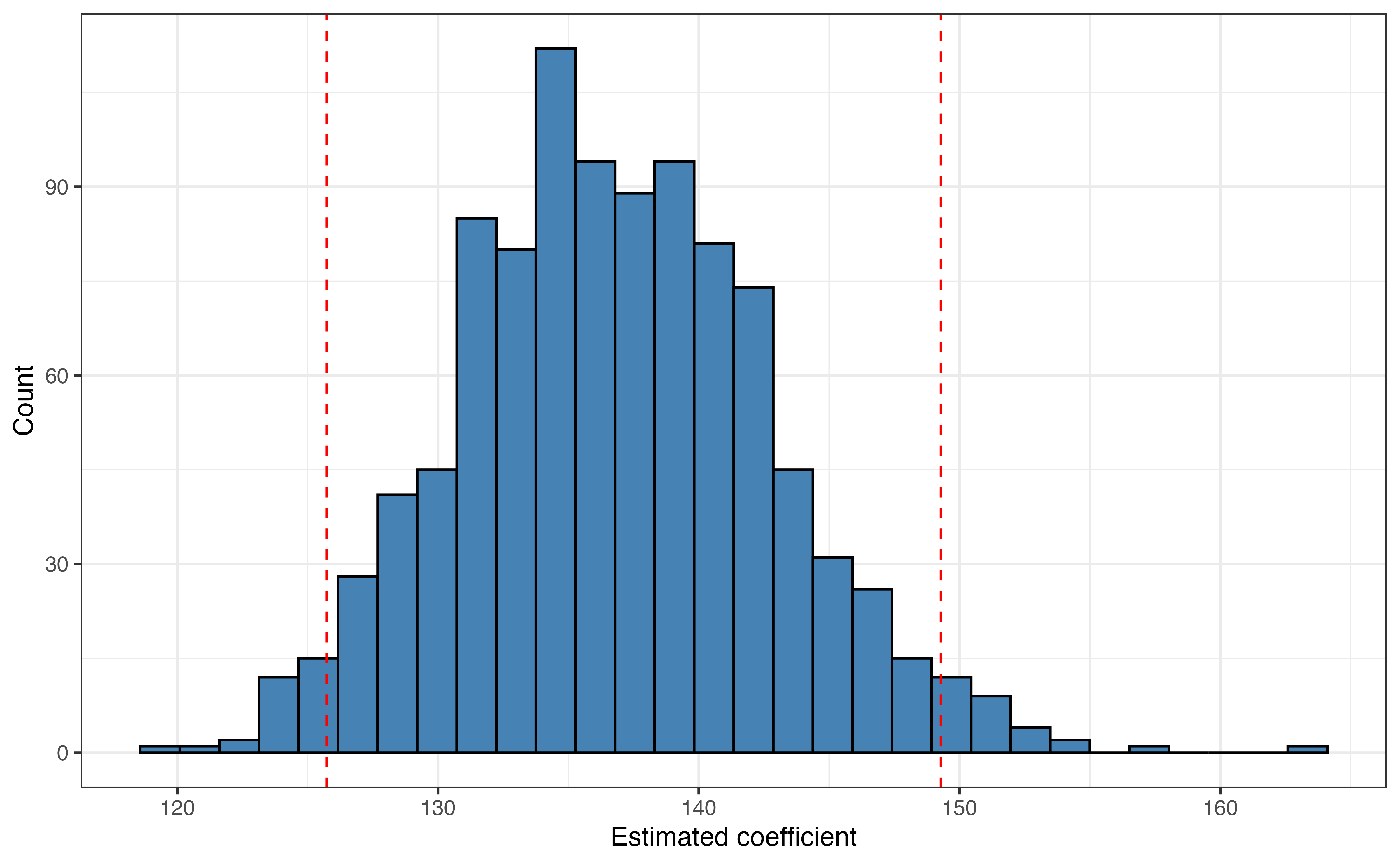
Figure 8.1 is the bootstrap sampling distribution for \(\hat{\beta}_{age}\). The mean of the distribution is 136.809 and the standard deviation is 5.97. The mean of the bootstrap distribution is very close to the estimated coefficient of age in the original model in Table 8.1. These values will not be exactly equal, because the bootstrap distribution is constructed from a simulation-based process that itself involves sampling. Given a confidence level \(C\), the \(C\%\) confidence interval is the middle \(C\%\) of the bootstrap distribution. \(C\) is generally set between 90 and 99, to balance accuracy and precision (see Section 5.4), with 95 being a commonly used default value.
Explain what 5.97 means in the context of the analysis.2
age with 95% confidence interval
Figure 8.2 shows the upper and lower bounds for a 95% confidence interval on the bootstrap sampling distribution. The 95% confidence interval for the \(\beta_{age}\), the coefficient of age is 125.74 to 149.29. Similar to the confidence interval in simple linear regression, we are 95% confident that this interval contains the true coefficient for age. Let’s interpret what this means in terms of the relationship between age and weight for young lemurs.
We are 95% confident that the weight of young lemurs increase between 125.74 and 149.29 grams, on average, for each additional month older, holding taxon, sex, and number of lemurs in the litter constant.
As before, the “confidence” referenced in this statement is the long-run confidence derived from the statistical process used to compute the interval. This means that if we repeat the process outlined in this section thousands of times, and thus have thousands of bootstrap distributions and confidence intervals, then about 95% of the confidence intervals would contain the true coefficient \(\beta_{age}\). Because we don’t know what \(\beta_{age}\) is (if we knew \(\beta_{age}\), we wouldn’t need inference!), we cannot state for certain whether the interval we computed is one of the 95% of intervals that contains the true coefficient or the 5% that miss the mark. Thus, we state in the interpretation that we are “95% confident”.
8.3.2 Permutation tests
Sometimes we wish to evaluate a claim made about the relationship between the response variable and one of the predictors, \(X_j\) using a hypothesis test. When conducting hypothesis tests to evaluate such a claim, the null hypothesis is the “baseline” condition of no linear relationship between the response and the predictor variable (\(H_0: \beta_j = 0\)) , and the alternative hypothesis is that there is a linear relationship (\(H_a: \beta_j \neq 0\)). Hypothesis tests can be used to evaluate other claims as well; however, we will focus on evaluating whether there is a linear relationship, because this is the claim being evaluated in output of most statistical software. See Section 5.5 for an introduction to hypothesis tests.
Section 5.6 provides an introduction more specifically to permutation tests, so here we will show how to conduct the test for multiple linear regression and answer the question posed in Section 8.1 :
Is age a useful predictor of weight, after accounting for sex, taxon, and number of lemurs in the litter?
We begin by stating the hypotheses in the context of the data:
- Null: There is no linear relationship between age and weight after accounting for sex, taxon, and number of lemurs in the litter.
- Alternative: There is a linear relationship between age and weight after accounting for sex, taxon, and number of lemurs in the litter.
The hypotheses in mathematical notation are the following:
\[ H_0: \beta_{age} = 0 \text{ vs. }H_a: \beta_{age} \neq 0 \]
In Section 5.5, we explained how hypothesis tests are conducted assuming null hypothesis is true, and the aim is to evaluate the strength of the evidence against the null hypothesis. Therefore, we need to obtain the sampling distribution of \(\hat{\beta}_{age}\) under the assumption that there is no linear relationship between age and weight, after accounting for the other predictors in the model. This sampling distribution is the null distribution, and we construct it using permutation sampling.
Permutation sampling is the process of shuffling one or more columns of data, to get many new combinations of the data, i.e., “new” samples. In this case, because we are conducting inference for a single predictor age, we will create new samples by shuffling the values of age, so that they are randomly paired with values of weight. We do not shuffle the columns of the other predictors, because we are evaluating the relationship between age and weight after accounting for the relationships between weight and the predictors sex, taxon, and litter_size. By shuffling the columns of age, we are simulating the null condition of no linear relationship between age and weight.
| weight | age | sex | taxon | litter_size | |
|---|---|---|---|---|---|
| Original Sample | 410 | 2.27 | F | ERUF | 0 |
| Permutation 1 | 410 | 20.52 | F | ERUF | 0 |
| Permutation 2 | 410 | 13.51 | F | ERUF | 0 |
| Permutation 3 | 410 | 16.41 | F | ERUF | 0 |
| Permutation 4 | 410 | 12.20 | F | ERUF | 0 |
| Permutation 5 | 410 | 22.06 | F | ERUF | 0 |
Table 8.4 shows the values from the original data and values from the first five permutations for an individual lemur. In the table, we see the values for weight, sex, taxon, and litter_size are the same for each permutation. The values of age are randomly shuffled, and there is no linear relationship (or any relationship) between age and weight in the permutation samples.
Like bootstrapping, each permutation sample is the same size as the original data. In contrast to bootstrapping, permutation sampling is merely shuffling the values of a column of data rather than sampling complete observations with replacement. We will use 1000 permutation samples for this analysis. Like bootstrapping, for each permutation sample, we fit the linear regression model and use \(\hat{\beta}_{age}\), the estimated coefficient of age from each permutation sample to create the null distribution.
- What is the approximate center of the null distribution of
agecreated from the permutation samples? - How does the standard deviation of the null distribution compare to the standard deviation of the bootstrap distribution?4
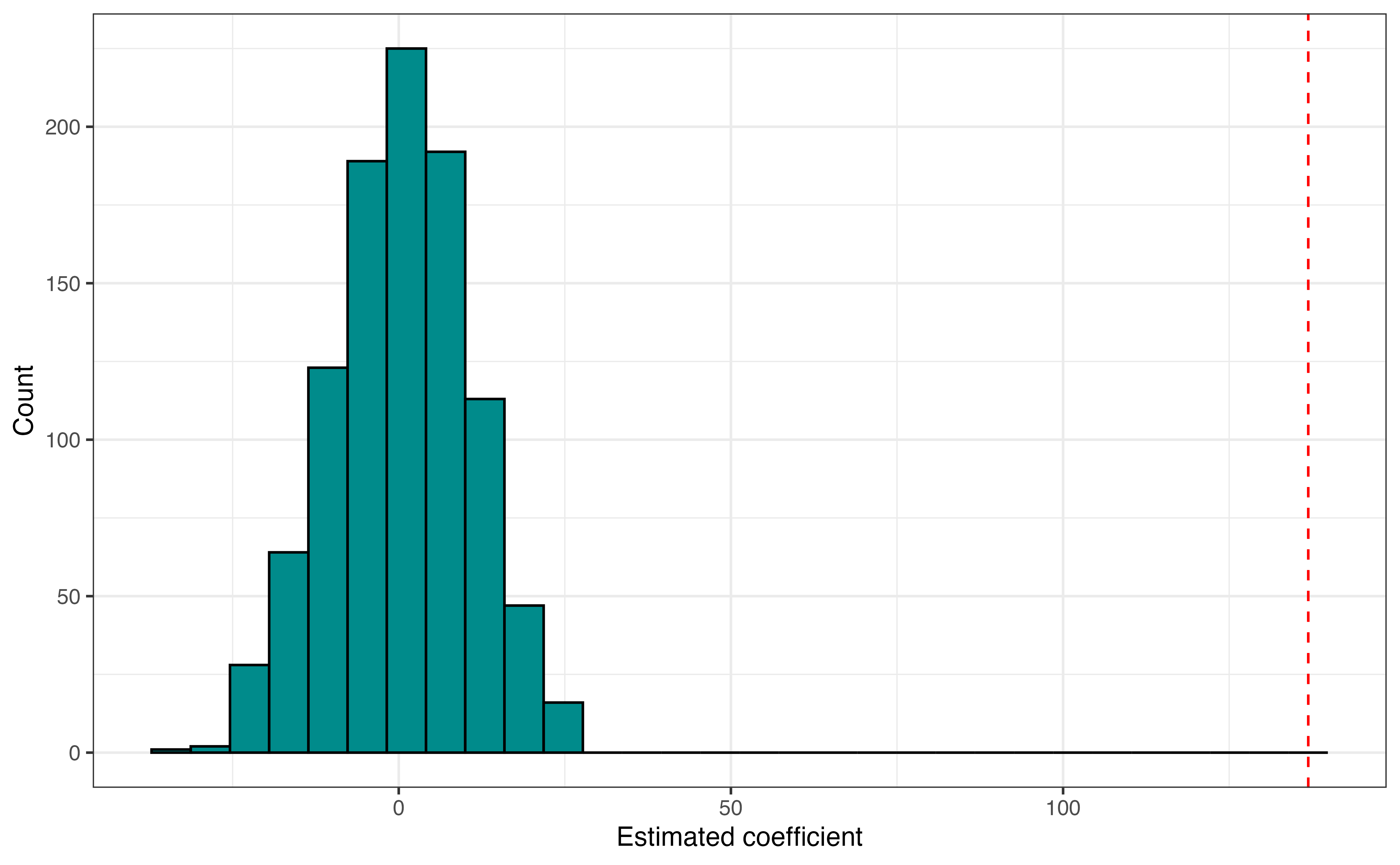
age from 1000 permutation samples
Figure 8.3 shows the null distribution with the value of \(\hat{\beta}_{age}\) observed in the original data marked with the red dotted line. The null distribution is centered around 0, the hypothesized value. The coefficient estimated from the observed data is very far away from the center of the distribution, so the data appears to provide strong evidence against the null hypothesis.
The evidence against the null hypothesis is not always so visually clear, so we compute a p-value to provide a measure for evaluating the evidence against the null hypothesis. Recall that the p-value is the probability of observing results at least as extreme as the results observed from the data, given the null hypothesis is true. In this instance, this means the probability of getting an estimated coefficient of 136.903 or more extreme in a sample of 252 lemurs, given the null hypothesis is true. Because the alternative hypothesis is \(\beta_{age} \neq 0\), “more extreme” is greater than 136.903 and less than -136.903 .
Based on the simulation, the p-value is 0. This means in 1000 permutation samples drawn under the assumption the null hypothesis is true, we did not compute an estimated coefficient for age equal to 136.903 or more extreme. We compare this p-value to a decision-making threshold \(\alpha\) (see Section 5.6.4) to draw the conclusion. The p-value of 0 is less than \(\alpha\) for any chosen threshold, so we reject the null hypothesis. The data provide strong evidence in favor of the alternative hypothesis that there is a linear relationship between age and weight after accounting for sex, taxon, and number of lemurs in the litter.
Though the p-value from the simulation-based hypothesis test is equal to 0, the true p-value is very close to but not exactly 0 (but it is still very small!). R will produce a warning like the one below to highlight this.

We can report such p-values as “approximately 0” to make clear to the reader that this is an approximation and not an exact result. We can also increase the number of iterations to get a closer approximation of the p-value or use theory-based methods from Section 8.4 to get the exact p-value.
Here we used permutation sampling to construct the null distribution for the hypothesis test to evaluate a claim about the relationship between age and weight for young lemurs. Because we conducted a two-sided hypothesis test, we can use the bootstrap confidence interval from Section 8.3.1 to evaluate this claim as well. The \(C\%\) confidence interval corresponds to a test with a decision-making threshold of \(\alpha = (1-\frac{C}{100})\). See Section 5.7 for more detail about the connection between hypothesis test and confidence intervals.
The 95% bootstrap confidence interval for \(\beta_{age}\) is 125.74 to 149.29.
- This interval corresponds to a hypothesis test with what \(\alpha\) -level?
- Is this interval consistent with the conclusion that there is evidence of a linear relationship between age and weight, after accounting for sex, taxon, and number of lemurs in the litter? Explain. 5
8.4 Theory-based inference
The other approach for inference is using theory-based methods based on mathematical models and the Central Limit Theorem. Theory-based methods have formulas to quantify the sampling variability in the estimated coefficient and uses distributions to compute exact confidence intervals and p-values. Because these methods rely on formulas rather than resampling methods, they are very computationally efficient. Results from theory-based inferential methods are displayed in the model output from most statistical software. For example, you can see the inferential results we’ll discuss in the model output in Table 8.1.
Theory-based inference for coefficients in a multiple linear regression model is very similar to inference in simple linear regression. Therefore, this section will provide a brief description of these methods, show how they apply to answer the questions in Section 8.1, and highlight differences from simple linear regression. See Section 5.8 for a thorough introduction to these methods. The mathematical details utilize linear algebra and are found in Section A.5 and Section A.6.
8.4.1 Foundations for inference
When doing multiple linear regression, we assume a model structure of the from in Equation 8.1.
\[ Y = \beta_0 + \beta_1X_1 + \beta_2X_2 + \dots + \beta_pX_p + \epsilon \hspace{8mm} \epsilon \sim N(0, \sigma^2_{\epsilon}) \tag{8.1}\]
The equation written in terms of the distribution of \(Y\) given a combination of predictors \(X_1, X_2, \ldots, X_p\) in Equation 8.2.
\[ Y|X \sim N(\beta_0 + \beta_1X_1 + \beta_2X_2 + \dots + \beta_pX_p, \sigma^2_{\epsilon}) \tag{8.2}\]
By Equation 8.2, the distribution of the response variable \(Y\) given a combination of predictors \(X_1, X_2, \ldots, X_p\) is normally distributed, centered at \(\beta_0 + \beta_1X_1 + \beta_2X_2 + \dots + \beta_pX_p\) with variance \(\sigma^2_{\epsilon}\). Based on this distribution, the following assumptions are made when we conduct multiple linear regression:
The distribution of the response \(Y\) is normal for a given combination of the predictors\(X_1, X_2, \ldots, X_p\).
The expected value (mean) of the distribution of \(Y\) given \(X_1, X_2, \ldots, X_p\) is \(\beta_0 + \beta_1 X_1 + \beta_2X_2 + \dots + \beta_pX_p\). There is a linear relationship between the response and the predictor variables.
The variance of the distribution of \(Y\) given \(X_1, X_2, \ldots, X_p\) is \(\sigma^2_{\epsilon}\). This variance is equal for all combination of predictors \(X_1, X_2, \ldots, X_p\) and does not depend on the predictors.
The error terms \(\epsilon\) are independent of one another. This also means the values of the response variable, and the observations more generally, are independent of one another.
Notice that these assumptions are generally the ones for simple linear regression in Section 5.3. The difference is that the assumptions about \(Y\) are made for a combination of predictors rather than a single predictor.
In Chapter 7, we showed how to compute \(\hat{\beta}_0, \hat{\beta}_1, \hat{\beta}_2, \ldots, \hat{\beta}_p\), the estimated model coefficients. The remaining parameter \(\sigma_{\epsilon}\), called the regression standard error, is the variability of the observations about the regression line. The distance between the observed values and the regression line (the predicted value of \(Y\) for a given combination of predictors) is the residual. Equation 8.3 shows how we use the residuals to estimate the regression standard error.
\[ \hat{\sigma}_{\epsilon} = \sqrt{\frac{\sum_{i=1}^n e_i^2}{n - p -1 }} = \sqrt{\frac{\sum_{i=1}^n (y_i - \hat{y}_i)^2}{n - p -1 }} \tag{8.3}\]
This is very similar to Equation 5.8, the equation to estimate the regression standard error in simple linear regression. The difference is the denominator, \(n - p - 1\), where \(p\) is the number of predictor terms. The value \(n - p - 1\) is the degrees of freedom, the number of observations available to understand variability about the regression line. This stems from the fact that we “use” \(p+1\) observations to estimate the model coefficients. In simple linear regression, there is one predictor, so \(p = 1\), and the degrees of freedom are \(n - 2\) as shown in Section 5.8.2. Let’s compute the degrees of freedom for the regression standard error associated with the model in Table 8.1. There are \(n =\) 252 observations in the data and \(p = 5\) terms for predictors in the model. (Note that even though taxon is a single predictor, we need to account for the fact there are two terms for taxon estimated in the model). The degrees of freedom are
\[ df = 252 - (5 + 1) = 252 - 5 - 1 = 246 \]
Thus, there are 246 degrees of freedom, i.e., observations available to understand variability about the regression line for the lemurs analysis.
The goal is to conduct inference for a model coefficient \(\beta_j\), so we ultimately need to estimate the sampling variability in the estimated coefficients \(\hat{\beta}_j\). This variability is measured by \(SE_{\hat{\beta}_j}\), the standard error of \(\hat{\beta}_j\). The formula to compute \(SE_{\hat{\beta}_j}\) in Equation 8.4 is more complex than in the case of simple linear regression, because we need to understand the sampling variability of \(\hat{\beta}_j\) in the context of a regression model that includes other predictors.
\[ SE_{\hat{\beta}_j} = j^{th} \text{diagonal element of }\hat{\sigma}_{\epsilon}(\mathbf{X}^\mathsf{T}\mathbf{X})^{-1} \tag{8.4}\]
Mathematical details for Equation 8.4 are in Section A.6. For now, we’ll focus on a conceptual understanding about why the standard error computed here may be different than the standard error for the same predictor variable in the case of simple linear regression. To illustrate this, let’s look at the standard error for age in a simple linear regression model and in the model in Table 8.1. The coefficient estimates and standard errors are printed side-by-side in Table 8.5.
age in simple and multiple linear regression modelss
| term | estimate | std.error |
|---|---|---|
| (Intercept) | 555 | 67.31 |
| age | 142 | 5.88 |
| term | estimate | std.error |
|---|---|---|
| (Intercept) | 24.2 | 93.63 |
| age | 136.9 | 4.86 |
| sexM | -88.8 | 68.00 |
| taxonPCOQ | 471.7 | 95.43 |
| taxonVRUB | 1037.3 | 133.91 |
| litter_size | -19.6 | 65.80 |
The estimated standard error for age in the simple linear regression model is 5.883 compared to 4.858 in the multiple linear regression model. In the case of multiple linear regression, the other predictors in the model are accounted for in two ways when computing \(SE_{\hat{\beta}{age}}\) . First the other predictors are accounted for when computing \(\hat{\sigma}_\epsilon\), as they are used to compute the \(\hat{y}_i\) in the Equation 8.3. Second, the other predictors are accounted for in \((\mathbf{X}^\mathsf{T}\mathbf{X})^{-1}\), as this matrix quantifies any relationship between the predictor variables (see Section A.6 for details). Thus, based on the models in Table 8.5, there is less sampling variability in \(\hat{\beta}_{age}\) after we account for the other potential predictors of weight.
In addition to estimating the sampling variability for model coefficients, by the Central Limit Theorem, we know the full sampling distribution of the model coefficient \(\hat{\beta}_j\) is normally distributed, with a mean at the true population coefficient \(\beta_j\) and variance \(SE_{\hat{\beta}_j}^2\), the standard error squared as shown in Equation 8.5. We use this distribution as the basis for conducting hypothesis tests and computing confidence intervals.
\[ \hat{\beta}_j \sim N(\beta_j, SE_{\hat{\beta}_j}^2) \tag{8.5}\]
8.4.2 Hypothesis tests
The hypothesis test in multiple linear regression follows the same steps as simple linear regression in Section 5.6.1:
- State the null and alternative hypotheses.
- Calculate a test statistic.
- Calculate a p-value.
- Draw a conclusion.
Using these steps, we’ll conduct a hypothesis test with decision-making threshold \(\alpha = 0.05\), to answer the question from Section 8.1:
Is age a useful predictor of weight, after accounting for sex, taxon, and number of lemurs in the litter?
Step 1: State the null and alternative hypotheses.
The null and alternative hypotheses are the same for theory-based inference as they are for simulation-based inference. Thus, the null and alternative hypotheses are the following:
- Null: There is no linear relationship between age and weight after accounting for sex, taxon, and number of lemurs in the litter.
- Alternative: There is a linear relationship between age and weight after accounting for sex, taxon, and number of lemurs in the litter.
These hypothesis in mathematical notation are the following:
\[ H_0: \beta_{age} = 0 \text{ vs. }H_a: \beta_{age} \neq 0 \]
Step 2: Calculate a test statistic.
We conduct hypothesis testing assuming the null hypothesis is true. Applying this to Equation 8.5, we assume that \(\hat{\beta}_{age} \sim N(0, SE_{\hat{\beta}_{age}})\). Let’s use this to compute the test statistic, the number of standard errors \(\hat{\beta}_{age}\), the coefficient estimated from the data, is from the hypothesized center of the distribution 0.
The test statistic for \(\hat{\beta}_{age}\) is
\[ T = \frac{\hat{\beta}_j - 0}{SE_{\hat{\beta}_j}} = \frac{136.903 - 0}{4.858} = 28.181 \]
This means that given the null hypothesis is true (\(\beta_{age} = 0\)) , the coefficient estimated from the model 136.903 is about 28.181 standard errors above the mean of the distribution.
The test statistic is 28.181. Do you think this provides evidence in support of or against the null hypothesis?6
Step 3: Calculate a p-value.
Sometimes the test statistic has a magnitude that is so small or so large that we can easily use it to draw conclusions about the test. There are many times, however, it is unclear what the conclusion should be based on the test statistic alone, so we compute a p-value and compare it to the decision-making threshold \(\alpha\) to make a conclusion.
The definition of the p-value is similar for theory-based inference as with simulation-based inference. The key difference is that we will compare the test statistic, instead of the estimated coefficient, against a distribution. Thus, the p-value is the probability of observing a test statistic in the distribution at least as extreme as the observed test statistic, assuming the null hypothesis is true.
Under the null hypothesis, the test statistic follows a \(t\) distribution with \(n- p-1\) degrees of freedom, \(T \sim t_{n-p-1}\) . The \(t\) distribution is used, instead of the standard normal distribution, to account for the extra variability that results from using the estimated regression standard error \(\hat{\sigma}_\epsilon\) to compute the standard error of the coefficient in Equation 8.4 (see Section 5.6.1 for more detail about \(t\) distribution). Because the alternative hypothesis is not equal to, we conduct a two-sided test and compute the p-value as \(P(|t| > |T|) = P(t < -|T|) + P(t > |T|)\), the probability of obtaining a test statistic with magnitude greater than the test statistic \(T\).
In the hypothesis test for \(\beta_{age}\), the p-value is computed as
\[ P(|t| > |28.181|) = P(t < -28.181) + P(t > 28.181) \]
using a \(t\) distribution with 246 degrees of freedom. Using statistical software, the p-value is equal to 5.563^{-79} \(\approx 0\). Now we have an exact p-value that was estimated to be 0 using the permutation test in Section 8.3.2.
Step 4: Draw a conclusion.
The final step is to make a conclusion by comparing the p-value to the predefined decision-making threshold, \(\alpha\). If the p-value is less than \(\alpha,\) the evidence against the null is sufficiently strong, so we reject the null hypothesis and conclude the alternative. Otherwise, the evidence against the null hypothesis is not sufficiently strong, so we fail to reject the null hypothesis.
When writing the conclusion, we indicate whether to reject or fail to reject the null hypothesis then state what that means in the context of the data. Thus, for the hypothesis test for age, the conclusion is as follows:
The p-value is less than \(\alpha = 0.05\), so we reject the null hypothesis. The data provide sufficient evidence of a linear relationship between age and weight, after accounting for sex, taxon, and number of lemurs in the litter.
8.4.3 Confidence intervals
In Section 8.3.1, we used bootstrapping to simulate the sampling distribution of \(\hat{\beta}_j\), and marked the bounds of the middle \(C\%\) of the distribution to make the \(C\%\) confidence interval. Here, we will use the mathematical results about the distribution of \(\hat{\beta}_j\) and compute the confidence intervals using an equation of the form
\[ \hat{\beta}_j \pm t^*_{n-p-1} \times SE_{\hat{\beta}_j} \tag{8.6}\]
where \(t^*_{n-p-1}\) is the critical value marking the middle \(C\%\) of the \(t\) distribution with \(n - p - 1\) degrees of freedom. Let’s construct a 95% confidence interval for age to answer the question posed in Section 8.1 :
After taking into account sex, taxon, and number of lemurs in the litter, about how much does a young lemur’s weight increase, on average, as they get older?
We have previously computed \(\hat{\beta}_{age}\) and \(SE_{\hat{\beta}_{age}}\), so we just need to compute the critical value \(t^*_{n-p-1}\) using statistical software. This critical value is the point on the \(t\) distribution with \(n-p-1\) degrees of freedom such that 95% of the distribution (area under the curve) is between \(-t^*_{n-p-1}\) and \(t^*_{n-p-1}\). In this analysis, the critical value to construct the 95% confidence interval for \(\beta_{age}\) using a \(t\) distribution with \(n-p-1\) degrees of freedom is 1.651.
Now we have all the components needed to compute the confidence interval using Equation 8.6. By using the formula, we translate the interval from standardized values to the original units of the model coefficient by rescaling (multiplying) by \(SE_{\hat{\beta}_j}\) and shift by \(\hat{\beta}_j\). Thus to get the bounds of the confidence interval from \(\pm 1.651\) to values in terms of grams of weight per month older, we have
\[ 136.903 \pm 1.651 \times 4.858 = [128.882, 144.924] \]
Thus, we are 95% confident that the interval 128.882 to 144.924 contains \(\beta_{age}\), the true slope for age.7 More specifically in terms of the question, this means we are 95% confident that after accounting for sex, taxon, and number of lemurs in the litter, the weight of young lemurs increases between 128.882 to 144.924 grams, on average, as the age increases by one month. Recall that the “confidence” referenced here is our confidence in the statistical methods. That if we were to repeat the process of collecting 252 observations, fitting the same model, and making a confidence interval for the coefficient of age, about 95% of those intervals will actually contain the population coefficient. We cannot say for certain, however, whether this individual interval does or does not contain the true population coefficient for age.
Confidence intervals typically have confidence levels between 90% and 99%. Suppose you are considering three possible confidence levels: 90%, 95%, and 99%.
Which confidence level will you choose to get the most accurate interval?
Which confidence level will you choose to get the most precise interval?8
8.5 Model conditions and diagnostics
The simulation- and theory-based inference methods rely on a set of assumptions about the relationship between the response and predictor variables in the population (Section 8.4.1). We are unable to check whether these assumptions truly hold in the population, so we use the sample data to evaluate whether they hold in the data using model conditions. We also use model diagnostics to assess whether there are outliers in the data that are having an out-sized influence on the model results. These model conditions and diagnostics are the same the ones for simple linear regression (Chapter 6) with some additional considerations for the multiple predictor variables. Here we will show the conditions and diagnostics applied to the lemur model. See Chapter 6 for a detailed introduction to these topics.
8.5.1 Model conditions
There are four model conditions that align with the assumptions outlined in Section 8.4. These conditions, commonly know by the mnemonic LINE, are the following:
- Linearity: There is a linear relationship between the response and predictor variables.
- Independence: The residuals are independent of one another.
- Normality: The distribution of the residuals is approximately normal.
- Equal variance: The spread of the residuals is approximately equal for all predicted values.
Linearity
In the context of multiple linear regression, the linearity condition means that the relationship between the response and the predictor variables can be adequately described using the linear regression model. When this is the case, the residuals \(y_i - \hat{y}_i\) captures random variability that stems from the fact that there are factors other than the ones in the model that explain variability in weight and the natural random differences in weight we’d expect in a group of lemurs. To examine this, we use a plot of the residuals versus predicted values. Ideally, the residuals are randomly scattered, indicating the systematic relationship between the response and predictor variables has been capture by the model. The linearity condition is important for simulation-based and theory-based inference, so any violations in linearity should be addressed before conducting inference.
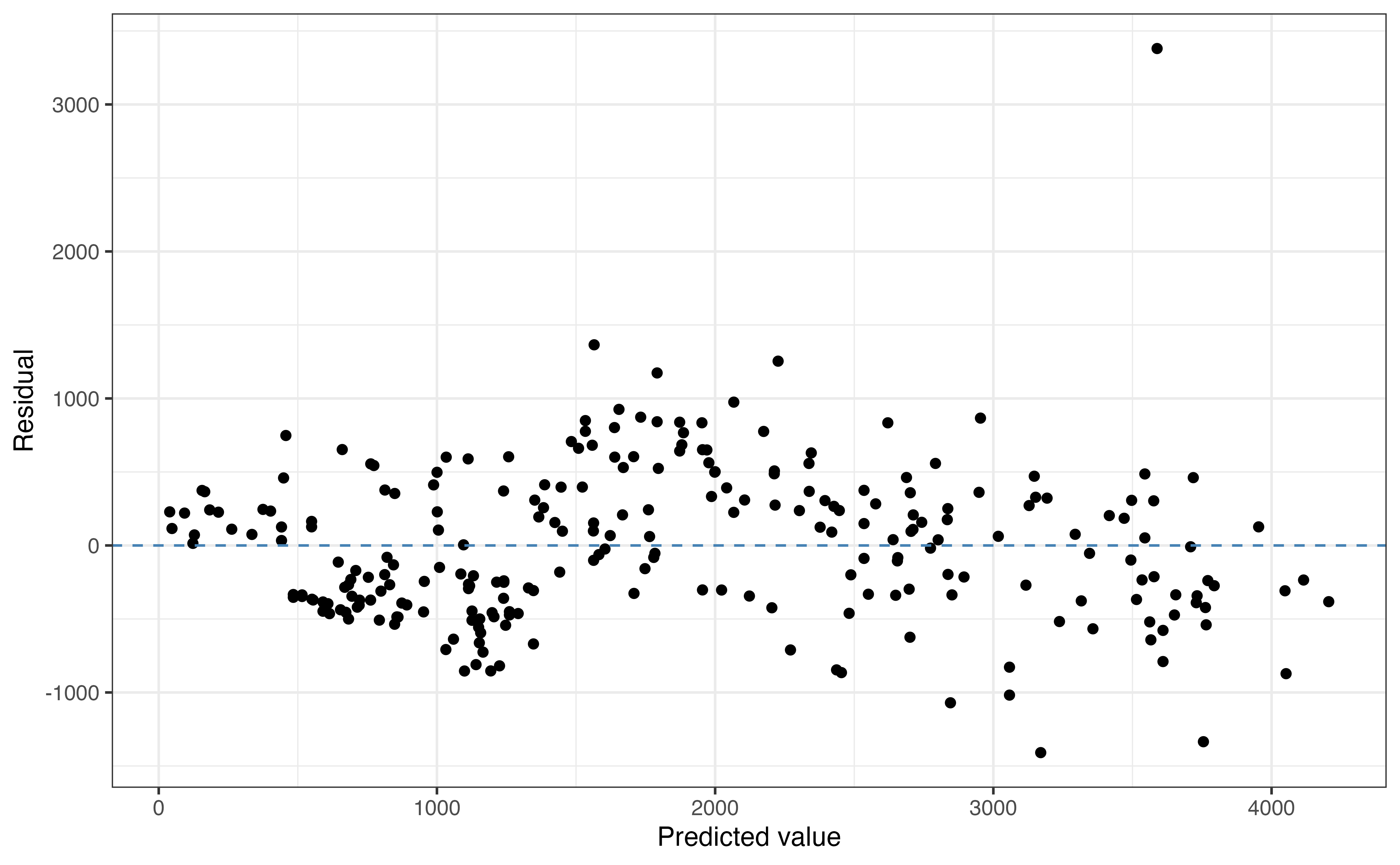
Based on Figure 8.4, the linearity condition is satisfied. The scatterplot shows no discernible pattern and the points are randomly scattered around \(\text{residual } = 0\). There is one point that stands out as an outlier with a large magnitude residual around 3500 grams. We will use model diagnostics to determine whether this outlier is, in fact, an influential point.
When the plot of residuals versus fitted values is randomly scattered as the one in this analysis, it is often sufficient to stop there when evaluating the linearity condition. If the plot of residuals versus predicted values shows some discernible pattern (for example, a parabola), we need to more closely examine the residuals versus each predictor variable to determine which variable has a non-linear relationship with the response. We may also choose to evaluate the residuals versus each predictor for more information about how well the model captures the underlying relationship with each predictor.
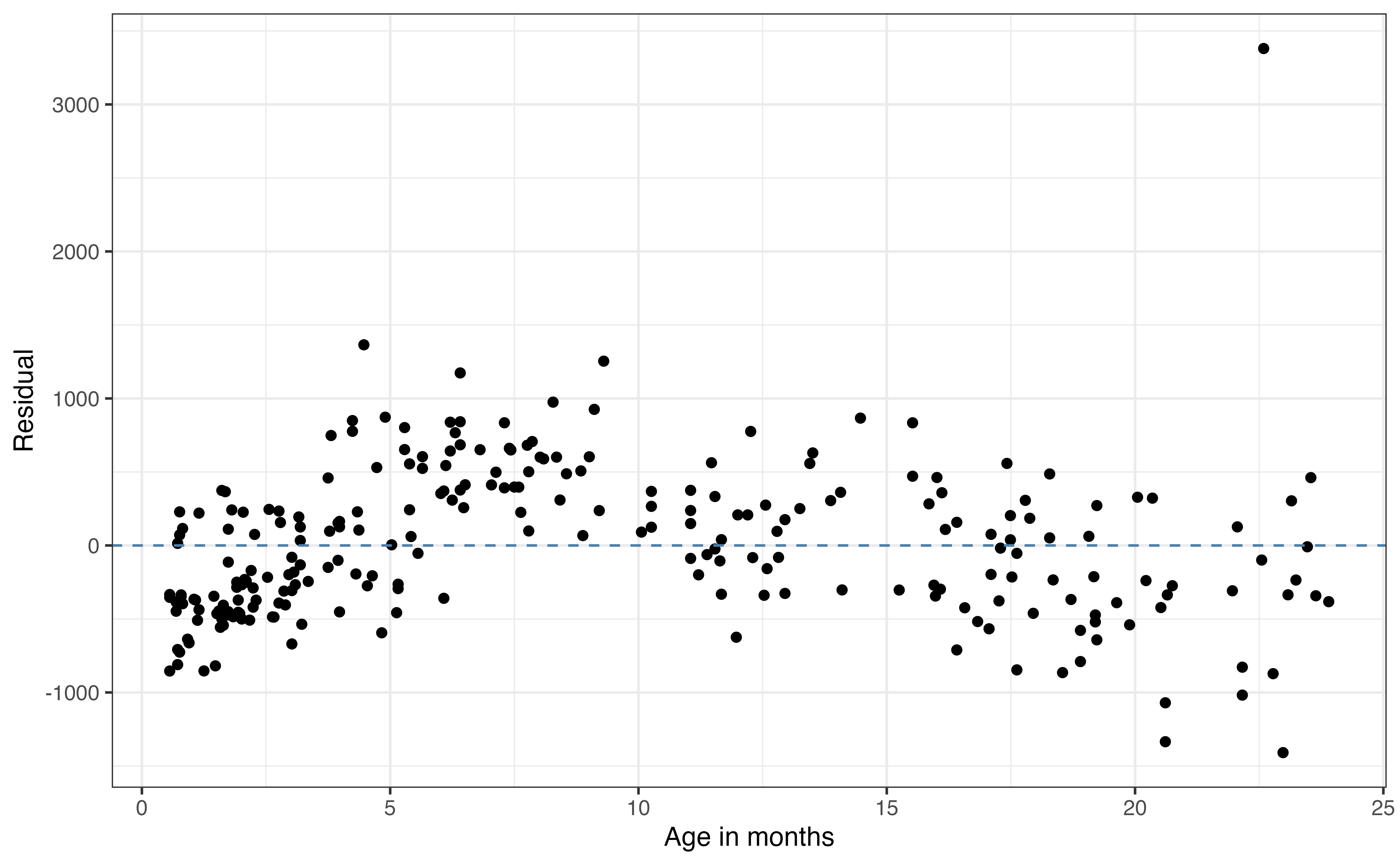
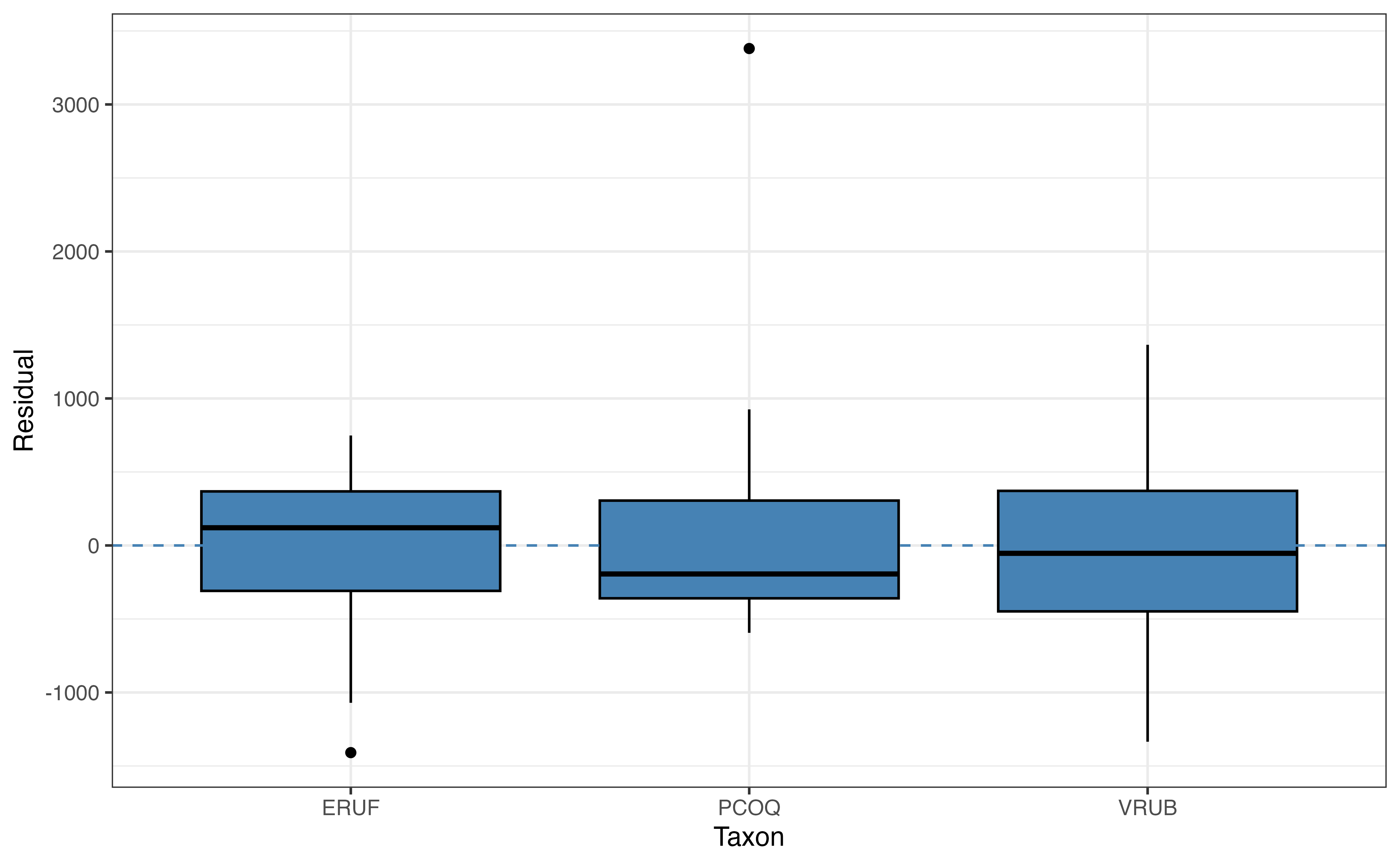
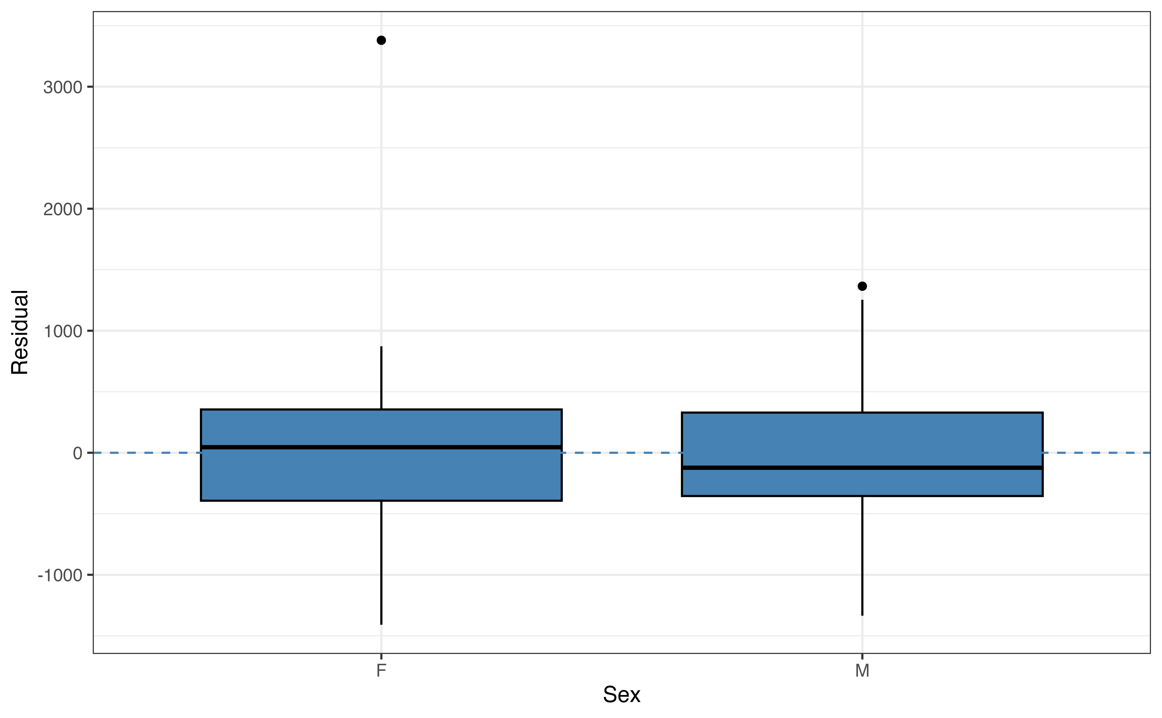
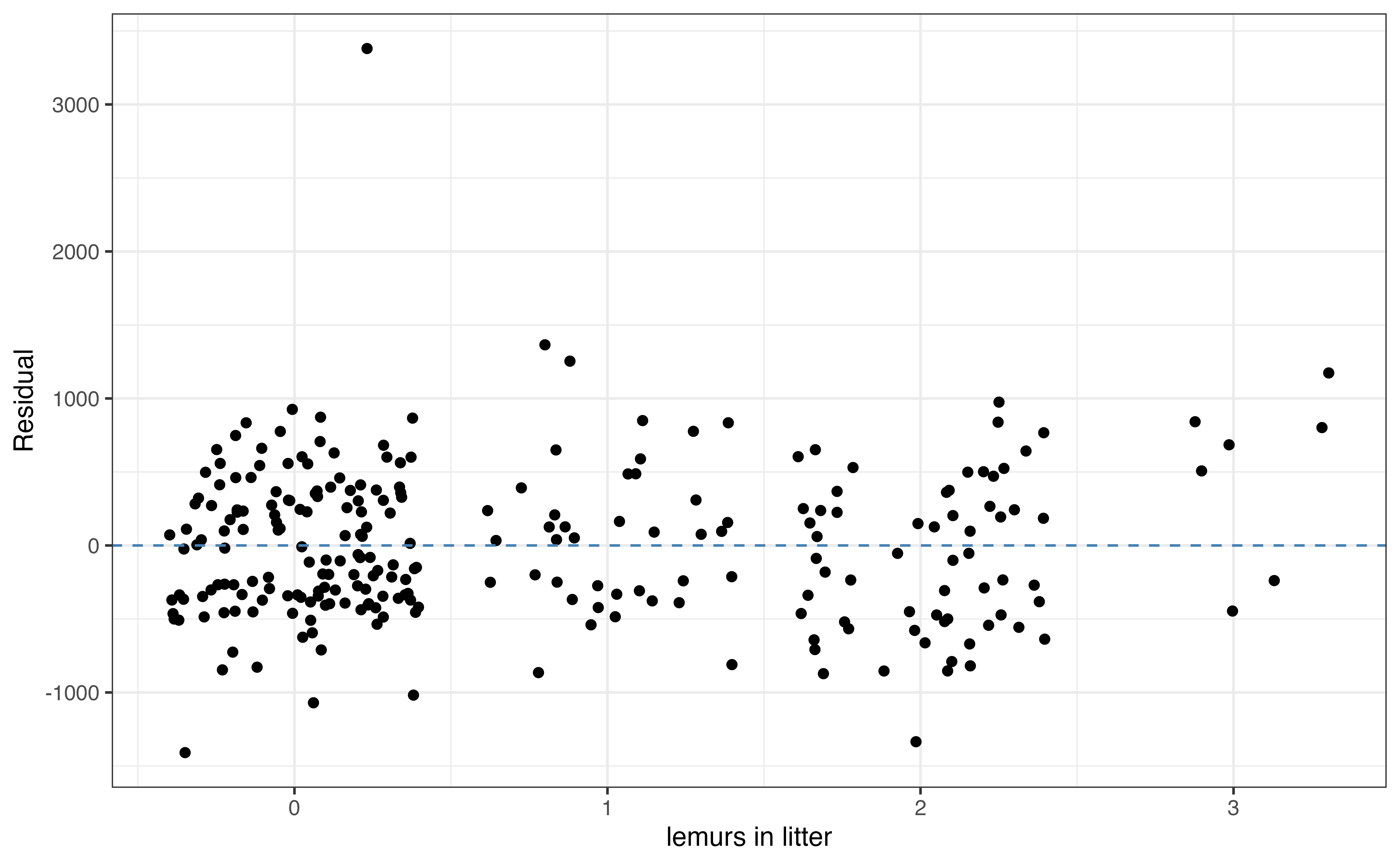
Figure 8.5 shows plots of the residuals versus each of the four predictor variables. We use the same criteria when evaluating the plots of residuals versus quantitative predictors. For example, the plot of residuals versus age in Figure 8.5 (a) shows there may be a non-linear relationships between age and weight. This is the same non-linearity we observed in the EDA in Section 7.1. Thus, we may consider using a transformed version of age in the model that more accurately represents the change in weight as age increases (see Chapter 9). We can then compare the model with the transformed age to the current model to determine which one is an overall better fit for the data. We discuss model comparison and selection in Chapter 10.
We use boxplots to examine the relationship between the response variable and categorical predictors. We expect the boxplots to be mostly vertically centered around \(\text{residual }=0\) for each category of a given predictor. For example, in the plot of taxon versus residual in Figure 8.5 (b), we see the center of each boxplot is close (though not exactly) equal to 0 and that in general the boxes for each taxon are spread around 0. One way to think about it is given a particular taxon, PCOQ for example, we cannot determine with almost any confidence whether the residual will be positive or negative. Therefore, the model sufficiently captures the relationship between taxon and weight. The same is true for sex in Figure 8.5 (c).
The residuals versus litter_size in Figure 8.5 (d) is randomly scattered, so the relationship between litter_size and weight is adequately captured in the model.
Independence
The next condition in LINE is independence. This condition is based on the assumption that the residuals are independent of one another; however, we often use information about the observations to evaluate this condition. As with simple linear regression, we use what we know about the subject matter and data collection process to evaluate whether it is reasonable to treat the observations as independent in the model. If the data have a time-ordered or spatial component, or were collected from subgroups not accounted for in the model, we can analyze the residuals to assess if there are violations in independence due to time or spatial correlation, or correlation with in a cluster.
Based on what we know about the lemur data, we can conclude that the independence condition is satisfied, and the observations can reasonably be treated as independent of one another. This means that the residuals for one lemur do not provide information about the residuals of another lemur.
The independence condition is important for simulation-based and theory-based inference, so any violations in independence should be addressed before conducting inference.
Normality
The next condition in LINE is normality. This condition is based on the assumption that the error terms are normally distributed, \(\epsilon_i \sim N(0, \sigma^2_{\epsilon})\). We we use a plot of the residuals to evaluate this claim.
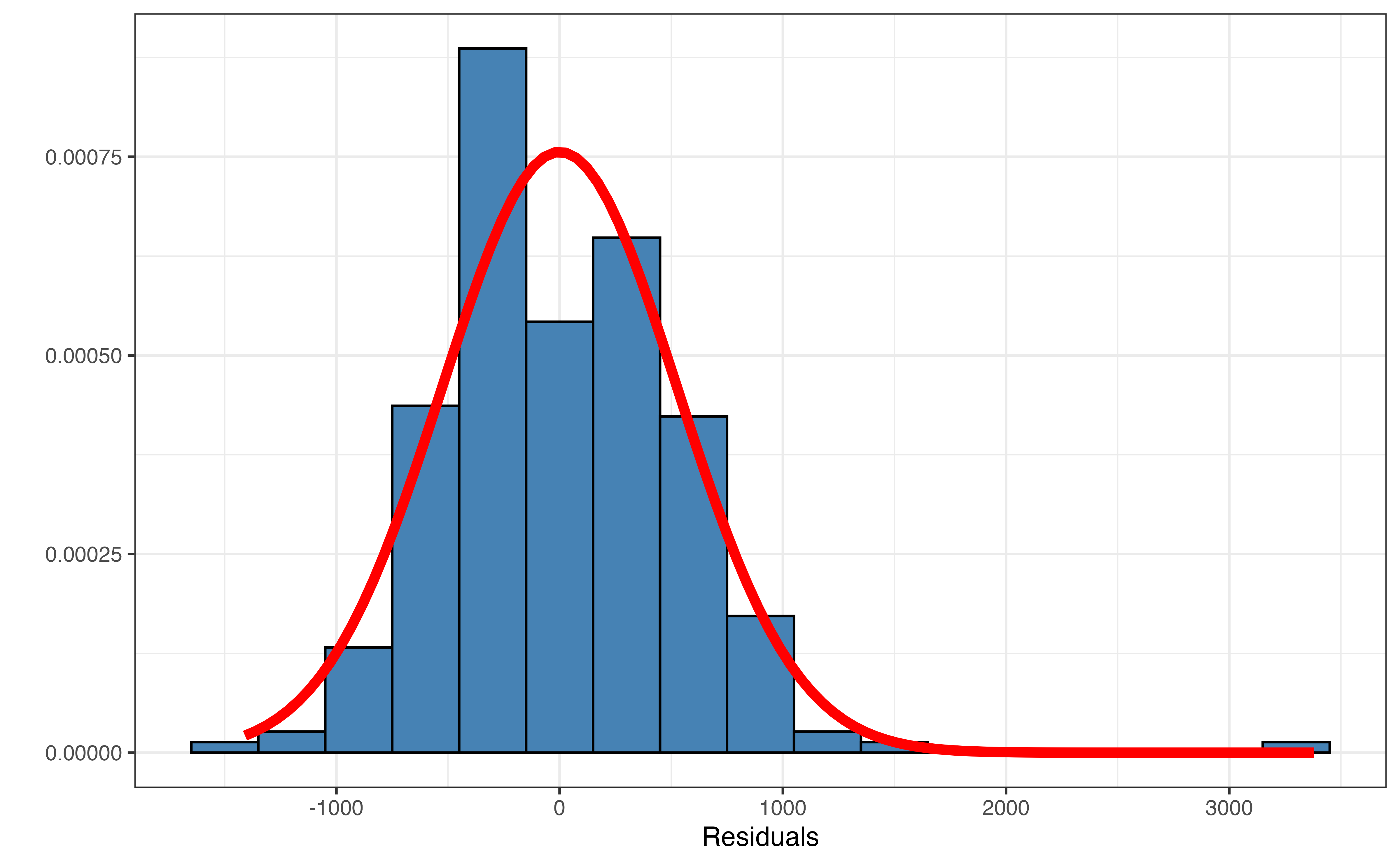
The distribution of the residuals with a normal curve applied is shown in Figure 8.6. We see the outlier with the large residual again in this plot. Focusing on the distribution without the outlier, the normal curve reasonably (though not perfectly) describes the distribution. Though not exactly, the distribution is approximately unimodal and symmetric, when the outlier is ignored. Therefore, we conclude the normality condition is satisfied.
Simulation-based inference does not rely on any assumptions about the distribution of the residuals, so it is robust to violations in the normality condition. From the Central Limit Theorem, theory-based methods for inference on the model coefficient are also robust to violations in normality when the sample is large enough. Typically 30 is used as the threshold for a “large enough” sample, but this value should not be treated as absolute. Thus, the closer the sample size is to 30, the closer the distribution of residuals needs to fit a normal distribution for reliable inferential results.
Equal variance
The final model condition in LINE is the equal variance condition. This condition comes from the assumption about the distribution of the error terms, \(\epsilon_i \sim N(0, \sigma^2_{\epsilon})\), that the variance in this distribution, \(\sigma^2_{\epsilon}\) is the same for all observations regardless of the values of the predictors. Thus, the variability of the residuals should be the same for all predicted values (combinations of predictors).
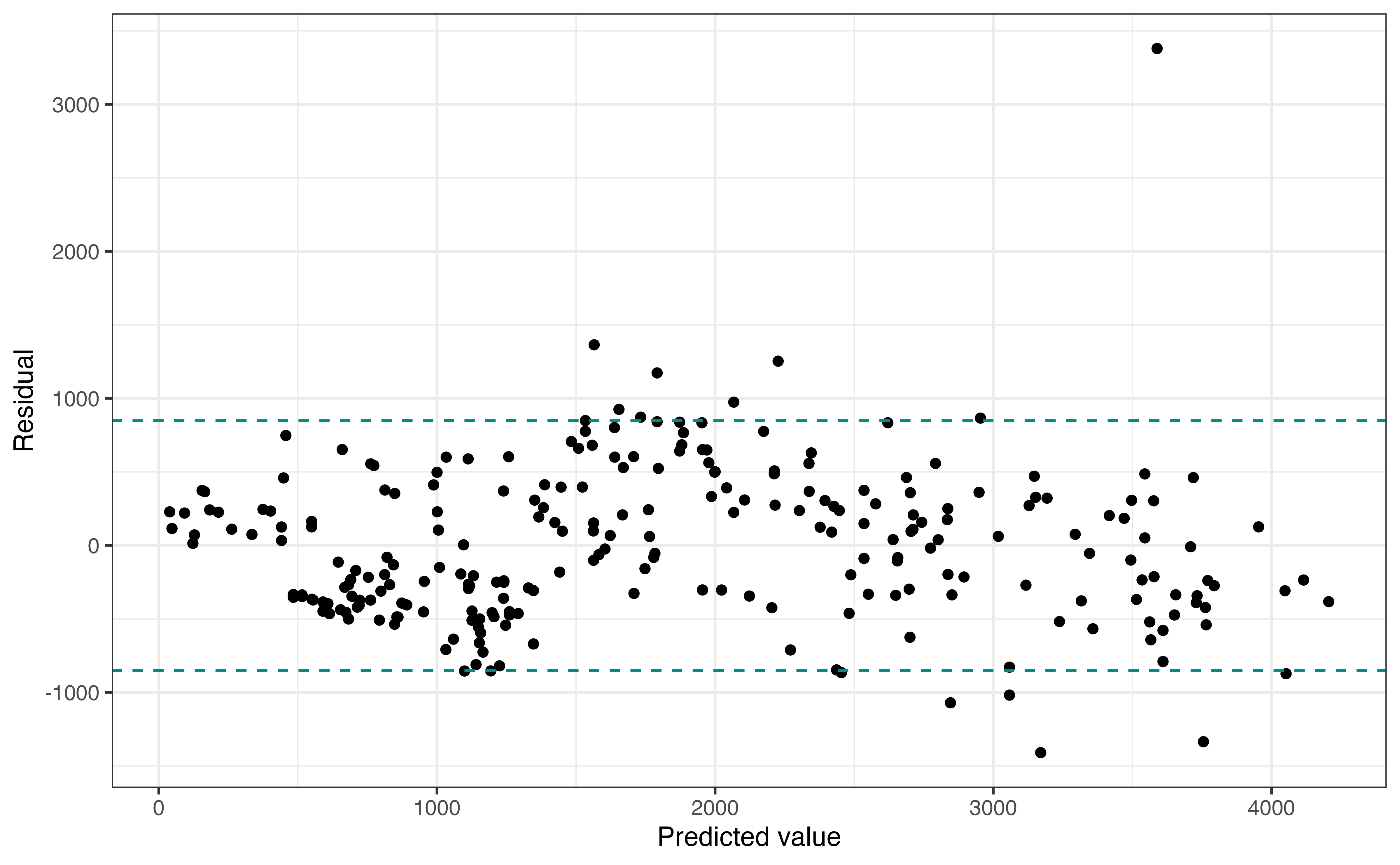
Figure 8.7 shows a plot of th residuals versus predicted values, similar to Figure 8.4. As we move along the \(x\)-axis, we are looking to see if the vertical spread is approximately equal for all observations. To help evaluate this, we have added vertical lines encompassing the majority of the data. Note as we move along the \(x\)-axis, the vertical spread fo the residuals is largely captured in by these vertical lines. Thus, the equal variance condition is satisfied. As with other conditions, we can ignore the high outlier when assessing the condition. Additionally, we are looking for noticeable violations in the conditions rather than perfect adherence when making the determination.
Simulation-based inference does not rely on any assumptions about the distribution of the residuals, so it is robust to violations in the equal variance condition. The regression standard error \(\hat{\sigma}_{\epsilon}\) is used to compute \(SE_{\hat{\beta}_j}\) in theory-based inference, so violations in the equal variance condition could lead to unreliable inference results. Therefore, any violations should be addressed before moving forward with inference. Chapter 9 introduces model transformations that can be used to address such violations.
8.5.2 Model diagnostics
After checking the model conditions, we evaluate model diagnostics to identify whether there are observations that have out-sized influence on the model. In Figure 8.4, we observed the outlying observation with the very large residual. Using model diagnostics, we can assess whether this observation is merely an outlier or, in fact, an influential point.
Cook’s distance
We begin by using Cook’s distance to determine whether there are influential points in the data.
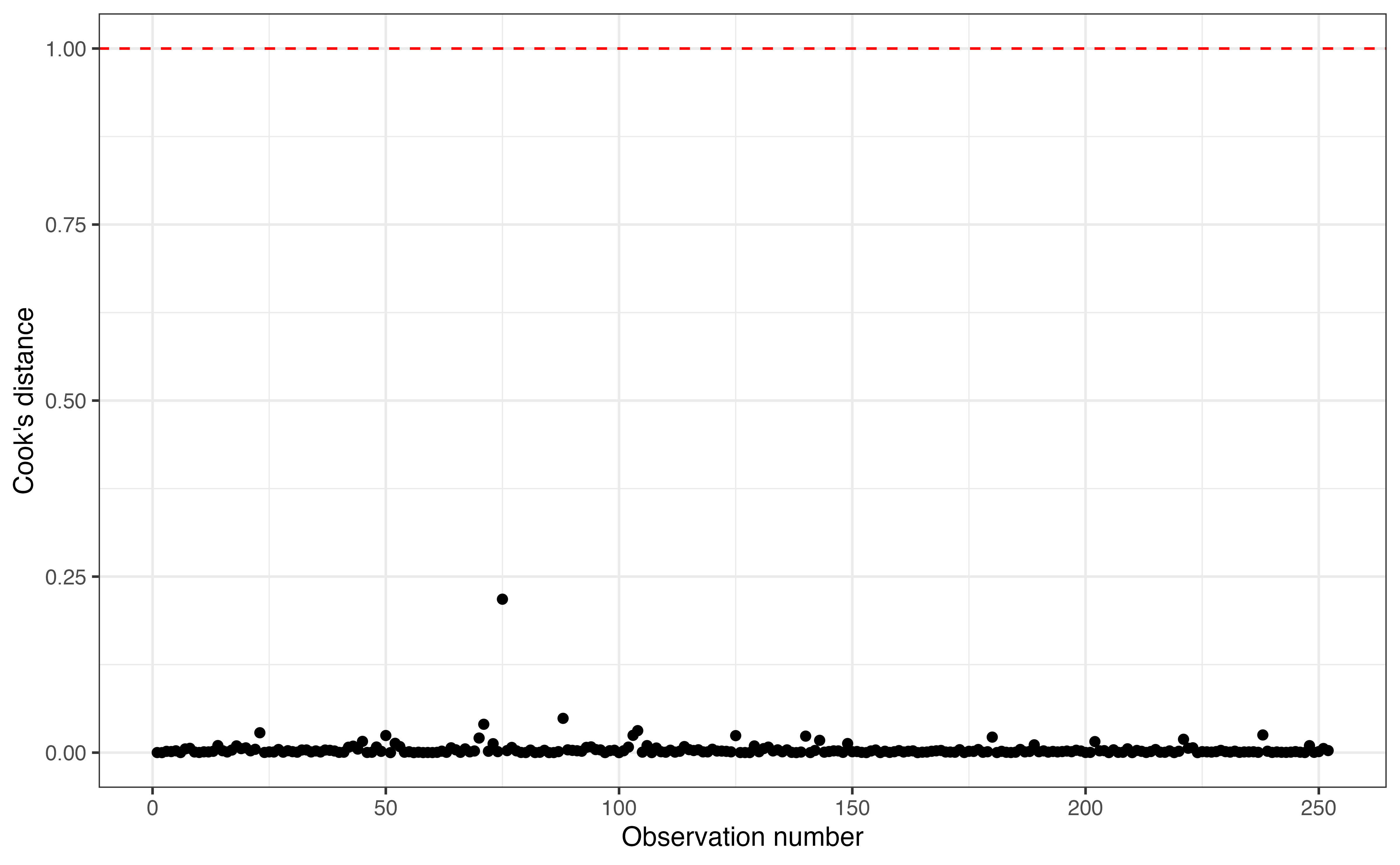
Figure 8.8 shows Cook’s distance for each observation. There is a horizontal line at \(\text{Cook's distance} = 1\) marking the threshold for influential observations. In this analysis, all the values of Cook’s distance are well below 1 (the maximum value is 0.218), so there are no influential points in the data. Thus, even though we have identified the an outlier, this observations did not have an out-sized impact on the estimated model coefficients.
Using the modeling workflow outlined in Section 6.5, if we have no influential points, we do not need to examine the components of Cook’s distance, leverage and standardized residuals. If we do identify an influential point, however, we can use leverage and standardized residuals to better understand how a given observation differs from the general trend of the data.
Though we did not find an influential point in this analysis, we will briefly discuss leverage and standardized residuals for multiple linear regression. See Section 6.4 for a introduction to these topics.
Leverage
In simple linear regression, an observation’s leverage is a measure of how far its value of the predictor is from the mean value of the predictor in the data. That definition is expanded in multiple linear regression, where an observation’s leverage is how far its combination of predictors is from the average (typical) combination of predictors. Mathematical details for computing leverage in multiple linear regression are in Section A.4.
Suppose we decide to fit a model using taxon, age, sex, and litter_size to predict the body length of young lemurs (instead of the weight)? How does the leverage for each observation compare in this model to the leverage in the model we’ve examined using these variables to predict weight?9
An observation has large leverage if its combination of predictors is far away from the typical combination in the data. We use a threshold of \(\frac{2(p+1)}{n}\), where \(p+1\) is the number of terms in the model and \(n\) is the sample size, to determine whether an observation has large leverage.
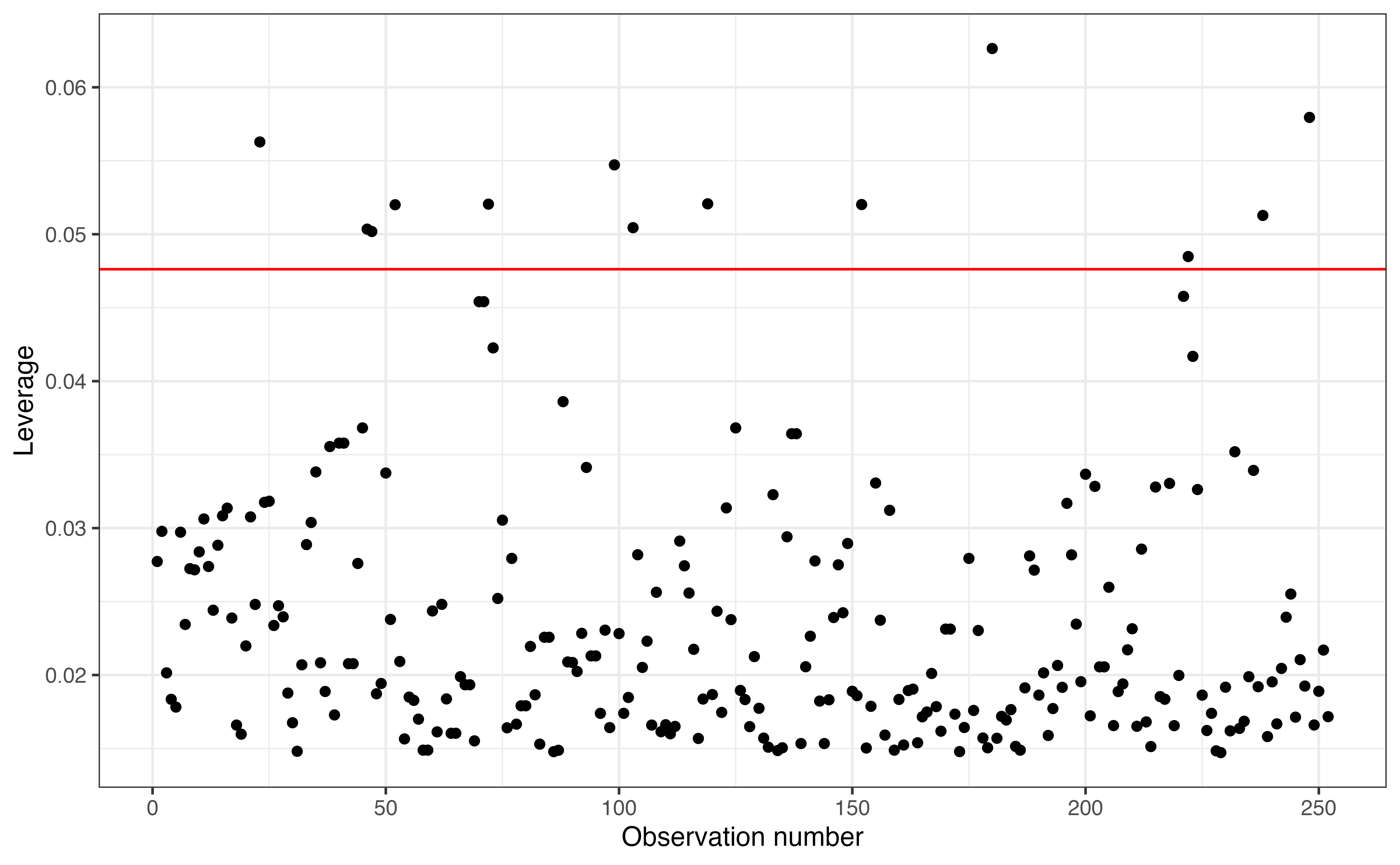
Figure 8.9 shows the leverage for each observation in the data. The leverage threshold 0.048 is marked on the graph. Based on this graph, there are 13 observations with large leverage. These are observations who have a combination of predictors that is far from the typical combination in the data. Given the multidimensionality of the data, it is not as straight forward to identify what makes these observations have large leverage as it was in simple linear regression. We can examine the data further to see what (if anything) these large leverage observations have in common and how they differ from the typical combination of predictors in the data. From Cook’s distance computed earlier; however, we know that these observations are not influential.
Standardized residuals
Standardized residuals are used to identify observations that have large magnitude residuals and thus the model poorly fit. We already noticed such an observation in Figure 8.4, so why do we need standardized residuals? Recall that residuals are on the same scale and have the same units as the response variable. Thus, if we use the raw residuals, we would need to determine a new threshold for identifying outliers in each analysis. On the other hand, standardized residuals are on the same scale in every analysis (mean of 0 and standard deviation of 1) with no units, so we can use a universal threshold that applies to every analysis.
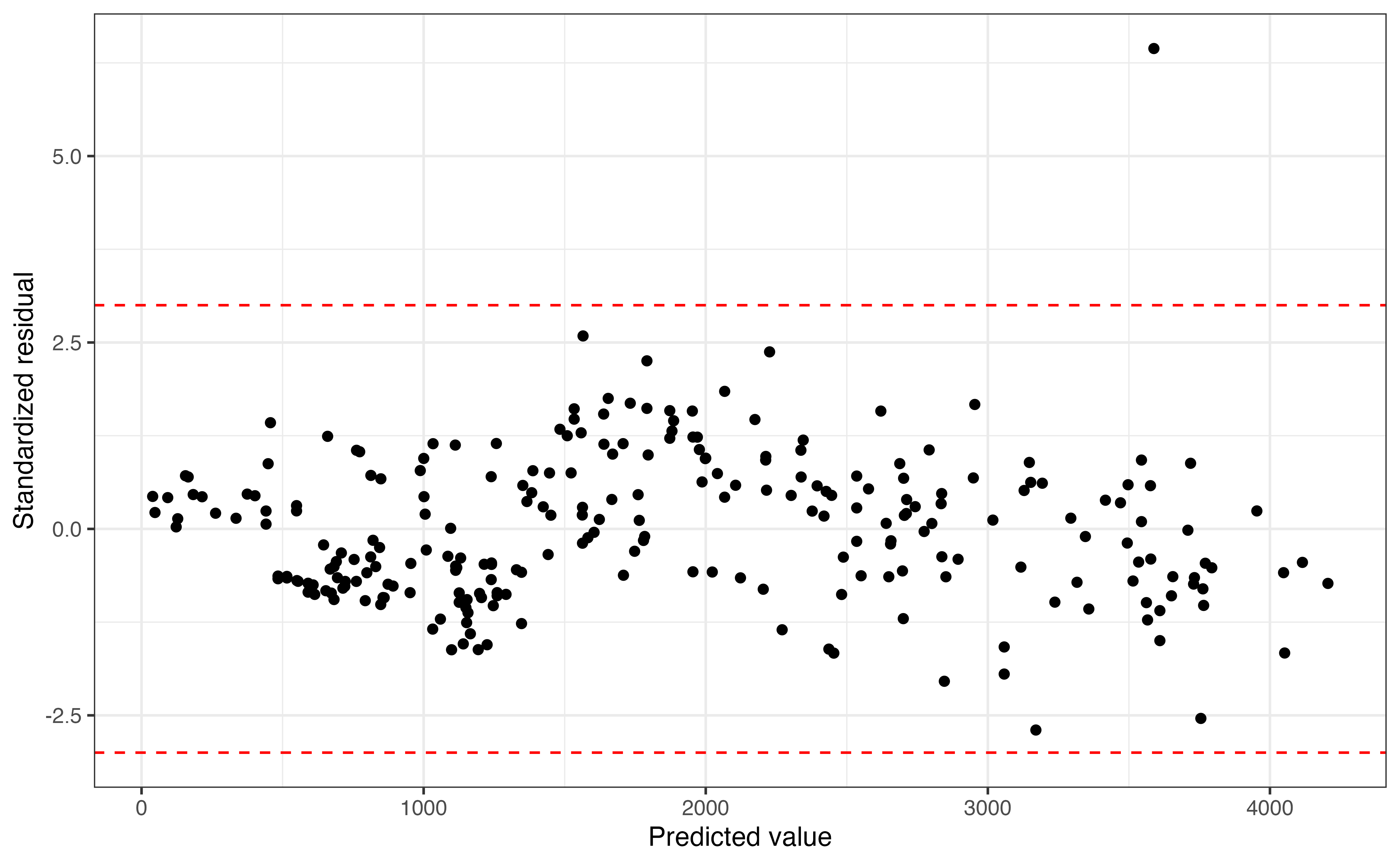
Figure 8.10 shows the standardized residuals versus predicted values, with lines at -3 and 3, the thresholds for identifying outliers. There is one observation that is an outlier in the \(Y\) direction with a standardized residual of 6.442. Though this observation is a noticeable outlier in the model performance, it is not an influential point based on Cook’s distance computed earlier.
Consider the outlier observation. The residual for this observation is 3380.42 and the standardized residual for this observation is 6.442.
- Explain what the value of the residual means in the context of the data.
- Explain what the value of the standardized residual means in the context of the data.10
We did not have any influential points in this analysis, but there will be times when do have such points in modeling. Section 6.4.5 discuses strategies for handling influential points in modeling.
8.6 Multicollinearity
8.7 Inference for multiple linear regression in R
8.7.1 Simulation-based inference in R
As with simulation-based inference for simple linear regression, we use the infer R package (Couch et al. 2021) for bootstrap confidence intervals and permutation tests. The code is shown below with brief explanations in the comments. It is described in Section 5.9.1 and Section 5.9.2.
The code to construct the 95% bootstrap confidence interval for the coefficient of age is shown below.
set.seed(1234)
niter = 1000

# construct bootstrap distribution
boot_dist <- lemurs_sample_young |>
  specify(weight ~ age + sex + taxon + litter_size) |>
  generate(reps = niter, type = "bootstrap") |>
  fit()

# compute 95% confidence interval for age
boot_dist |>
  filter(term == "age") |>
get_confidence_interval(level = 0.95, type = "percentile")
# A tibble: 1 × 2
lower_ci upper_ci
<dbl> <dbl>
1 127. 149.Next, the code to construct the null distribution and compute p-value for the permutation test is below. Note that the argument variables = age is used in generate() to specify that age is the only column that is permuted (shuffled). The default for generate() is to permute all columns.
set.seed(12345)
niter = 1000

age_coef <- lemurs_model |>
  tidy() |>
  filter(term == "age") |>
  pull(estimate)

# construct null distribution
null_dist <- lemurs_sample_young |>
  specify(weight ~ age + sex + taxon + litter_size) |>
  hypothesize(null = "independence") |>
  generate(reps = niter, type = "permute", variables = age) |>
  fit()

# compute p-value
null_dist |>
  filter(term == "age") |>
  get_p_value(obs_stat = age_coef, direction = "two-sided")
Warning: Please be cautious in reporting a p-value of 0. This result is an approximation
based on the number of `reps` chosen in the `generate()` step.
ℹ See `get_p_value()` (`?infer::get_p_value()`) for more information.# A tibble: 1 × 1
p_value
<dbl>
1 08.7.2 Theory-based inference in R
The statistics associated with the hypothesis test for each coefficient are produced by default when printing the output using tidy(). We can add the arguments conf.int = and conf.level = to the tidy function to output the confidence interval for each model coefficient.
Below is the code to fit and output the model from Section 8.1 with the 95% confidence interval for the model coefficients. The kable function is used to display the results in a neatly formatted table rounding all values to three digits.
lemurs_model <- lm(weight ~ age + sex + taxon +
                          litter_size,
                        data = lemurs_sample_young)

tidy(lemurs_model, conf.int = TRUE, conf.level = 0.95) |>
kable(digits = 3)| term | estimate | std.error | statistic | p.value | conf.low | conf.high |
|---|---|---|---|---|---|---|
| (Intercept) | 24.2 | 93.63 | 0.259 | 0.796 | -160 | 208.7 |
| age | 136.9 | 4.86 | 28.182 | 0.000 | 127 | 146.5 |
| sexM | -88.8 | 68.00 | -1.306 | 0.193 | -223 | 45.1 |
| taxonPCOQ | 471.7 | 95.43 | 4.943 | 0.000 | 284 | 659.7 |
| taxonVRUB | 1037.3 | 133.91 | 7.747 | 0.000 | 774 | 1301.1 |
| litter_size | -19.6 | 65.80 | -0.298 | 0.766 | -149 | 110.0 |
8.7.3 Model conditions and diagnostics
We use the augment function to produce a tibble of the statistics used for model conditions and diagnostics as with simple linear regression. See Section 6.6 for a description of the output produced by augment() and how these values are used to check model conditions and diagnostics.
lemur_aug <- augment(lemurs_model)

lemur_aug |>
  slice(1:5)
# A tibble: 5 × 11
weight age sex taxon litter_size .fitted .resid .hat .sigma .cooksd
<dbl> <dbl> <chr> <chr> <dbl> <dbl> <dbl> <dbl> <dbl> <dbl>
1 410 2.27 F ERUF 0 335. 75.0 0.0277 534. 0.0000968
2 137 0.72 F ERUF 0 123. 14.2 0.0298 534. 0.00000374
3 206 0.69 F PCOQ 0 590. -384. 0.0201 533. 0.00182
4 185 1.05 M PCOQ 0 551. -366. 0.0183 533. 0.00150
5 373 2.66 F PCOQ 0 860. -487. 0.0178 533. 0.00257
# ℹ 1 more variable: .std.resid <dbl>8.8 Summary
In this chapter, we built upon inference for simple linear regression introduced Chapter 5 and showed how inference can be used to draw conclusions about model coefficients in multiple linear regression models. We showed how to conduct simulation-based inference using bootstrapping for confidence intervals and permutation tests for hypothesis testing. Then, we showed how to compute the values shown the regression output by conducting inference using mathematical models based on the Central Limit Theorem. Lastly, we showed how to check model conditions and diagnostics for multiple linear regression, building off of the introduction to these topics in Chapter 6.
Sometimes the data shows violations in the model conditions that need to be addressed to make reliable conclusions and predictions from the model. In the next chapter, we will introduce variable transformations that can be used to address violations in the model conditions, particularly in the linearity and equal variance conditions.
Question 1: This can be answered by hypothesis test and confidence interval. Question 2: This question can be answered by a confidence interval.↩︎
It is estimate of \(SE_{\hat{\beta}_{age}}\), the standard error of the coefficient of
age.↩︎We are 90% confident that the weight of PCOQ lemurs is 314.442 to 630.842 grams higher, on average, compared the weight of ERUF lemurs, holding age, sex, and litter size constant.↩︎
- The center of the null distribution is approximately equal to 0, the hypothesized value. Because the null is created using a simulation-based procedure, it will not be exact but very close as the number of samples increases.
- The standard deviation of the null distribution is approximately equal to the standard deviation of the bootstrap distribution. They are both approximations of \(SE_{\hat{\beta}_{age}}\).
It corresponds to a hypothesis test with \(\alpha = 0.05\). Yes, the interval is consistent, because the null hypothesized value 0 is not in the interval.↩︎
This is a large test statistic, so it appears to provide evidence against the null hypothesis. We will complete the last two steps of hypothesis testing to see the conclusion.↩︎
Our calculations do not exactly match the confidence interval produced by software, because we have used rounded values of the estimated slope, critical value, and standard error.↩︎
The confidence level 99% produces the most accurate interval. The confidence level 90% produces the most precise interval.↩︎
The leverage of each observation will be the same for the two models. Leverage only depends on the predictor variables. It does not depend on the response variable.↩︎
The residual means that the observed weight for this lemur is 3380.42 grams greater than the weight predicted by the model. The standardized residual means that the residual for this observation is 6.442standard errors above the mean of the distribution of residuals.↩︎