11 Logistic regression

Learning goals

Identify whether linear or logistic regression is appropriate for a given analysis
Calculate and interpret probabilities, odds, and odds ratios
Interpret the coefficients of a logistic regression model
Conduct simulation-based and theory-based inference for the coefficients of a logistic regression model
Evaluate model conditions for logistic regression
Conduct logistic regression using R

11.1 Introduction: Comfort with driverless cars

Artificial Intelligence (AI) has quickly become ubiquitous, with generative AI tools such as ChatGPT being widely adopted in the workplace, school, and throughout every day life. One area in particular where AI is continuing to grow is in self-driving cars. The notion of riding in car that drives around as an individual reads a book has increasingly become a reality, with some cities already having self-driving taxis on the road. Waymo, a company that deploys a fleet self-driving taxis (called “robotaxis”), describes its robotaxi as “the world’s most experienced driver.” and is operating in five United States cities with plans to expand to two more at the time of this writing. (waymo.com). Additionally, Amazon has launched a robotaxi service in Las Vegas called Zoox (Liedtke 2025).

Despite the growth of self-driving cars, there are still complex moral questions Vemoori (2024) and the general readiness individuals have with this new technology and driving experience. David LI, co-founder of Hesai, a remote-sensing technology company, said that the adoption of self-driving cars are not just a question about technology development, but “it is a social question, it is a regulatory question, it is a political question” (White 2025). Therefore, it is important to understand how people, some of who may already will one day purchase a self-driving car, view this technological phenomenon.

The goal of the analysis in this chapter is to use data from the 2024 General Social Survey (GSS) to explore individual characteristics associated with one’s comfort with self-driving cars.

The GSS, administered by the National Science Foundation and is administered by National Opinion Research Center (NORC) at the University of Chicago, began in 1972 and is conducted about every two years to measure “trends in opinions, attitudes, and behaviors” among adults age 18 and older in the United States (Davern et al. 2025). Households are randomly selected using multistage cluster sample based on data from the United States Census.

Respondents in the 2024 survey were part of the second year of an experiment studying survey administration and randomly split into two groups. The first group had the opportunity to complete the survey through an in-person interview (format traditionally used) and non-respondents were offered the online survey. The second group had the opportunity to take the online survey first, then non-respondents were offered the in-person interview.

The data are in gss24-ai.csv. The data were obtained through the gssr R package (Healy 2023). Questions about opinions on special topics such as technology are not given to every respondent, so the data in this analysis includes responses from 1521 adults who were asked about comfort with self-driving cars and who provided their age and sex in the survey. We will focus on the variables below (out of the over 600 variables in the full General Social Survey). The variable definitions are based on survey prompts and variable definitions in the General Social Survey Documentation and Public Use File Codebook (Davern et al. 2025).

For the remainder of the chapter, we will refer to self-driving cars as “driverless cars” to align with the language used in the 2024 GSS.

aidrive_comfort: Indicator variable for respondent’s comfort with driverless (self-driving) cars. 0: Not comfortable at all; 1: At least some comfort.
- This variable was derived from responses to the original survey prompt: “Comfort with driverless cars”. Scores ranged from 0 to 10 with 0 representing “totally uncomfortable with this situation” and 10 representing “totally comfortable with this situation”. Responses of 0 on the original survey were coded as aidrive_comfort = 0. All other responses coded as 1.
tech_easy : Response to the question, “Does technology make our lives easier?” Categories are Neutral, Can't choose (Respondent doesn’t know / is unable to provide an answer), Agree, Disagree.
tech_harm: Response to the question, “Does technology do more harm than good?”. Categories are Neutral, Can't choose (Respondent doesn’t know / is unable to provide an answer), Agree, Disagree.
age: Respondent’s age in years
sex: Respondent’s self-reported sex. Categories are Male, Female, the options provided on the original survey.
income: Response to the question “In which of these groups did your total family income, from all sources, fall last year? That is, before taxes.” Categories are Less than $20k, $20-50k, $50-110k, $110k or more, Not reported .
- Note: These categories were defined based on the 27 categories in income16 from the original survey.
polviews: Response to the question, “I’m going to show you a seven-point scale on which the political views that people might hold are arranged from extremely liberal–point 1–to extremely conservative–point 7. Where would you place yourself?” Categories are Moderate, Liberal, Conservative, No reported.
- Note: These categories were defined based on the original 7 point scale.

The General Social Survey includes sample weights, so that the analysis data is representative of the population of adults in the United States.

These sample weights are not used in the analysis in this chapter or Chapter 12 which uses the same data. Therefore, the analysis and conclusions we draw are only for educational purposes. To use the General Social Survey for research, see (Davern et al. 2025) for more information about incorporating the sample weights.

11.1.1 Exploratory data analysis

(a) Distribution of original resposnes from 2024 GSS

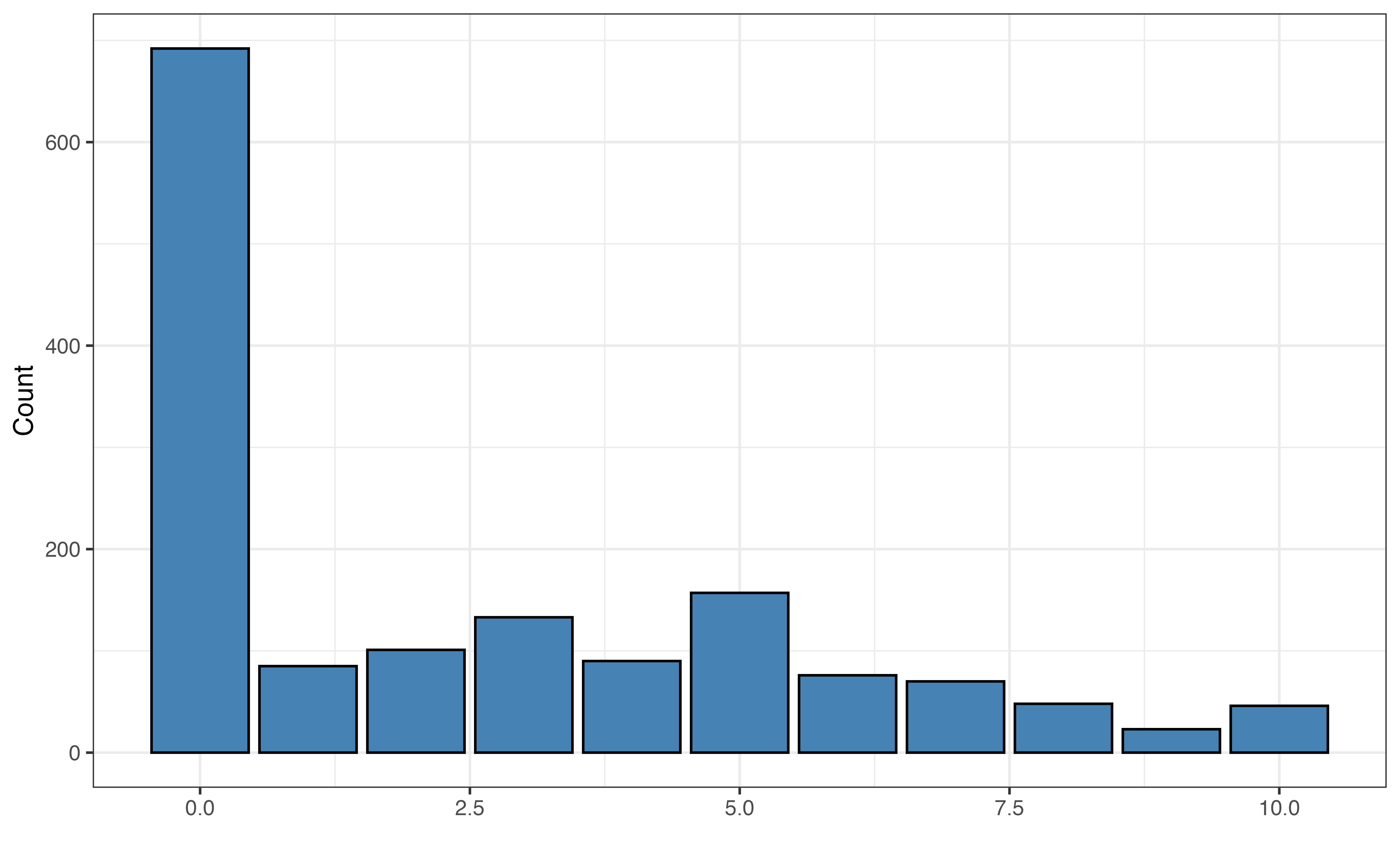
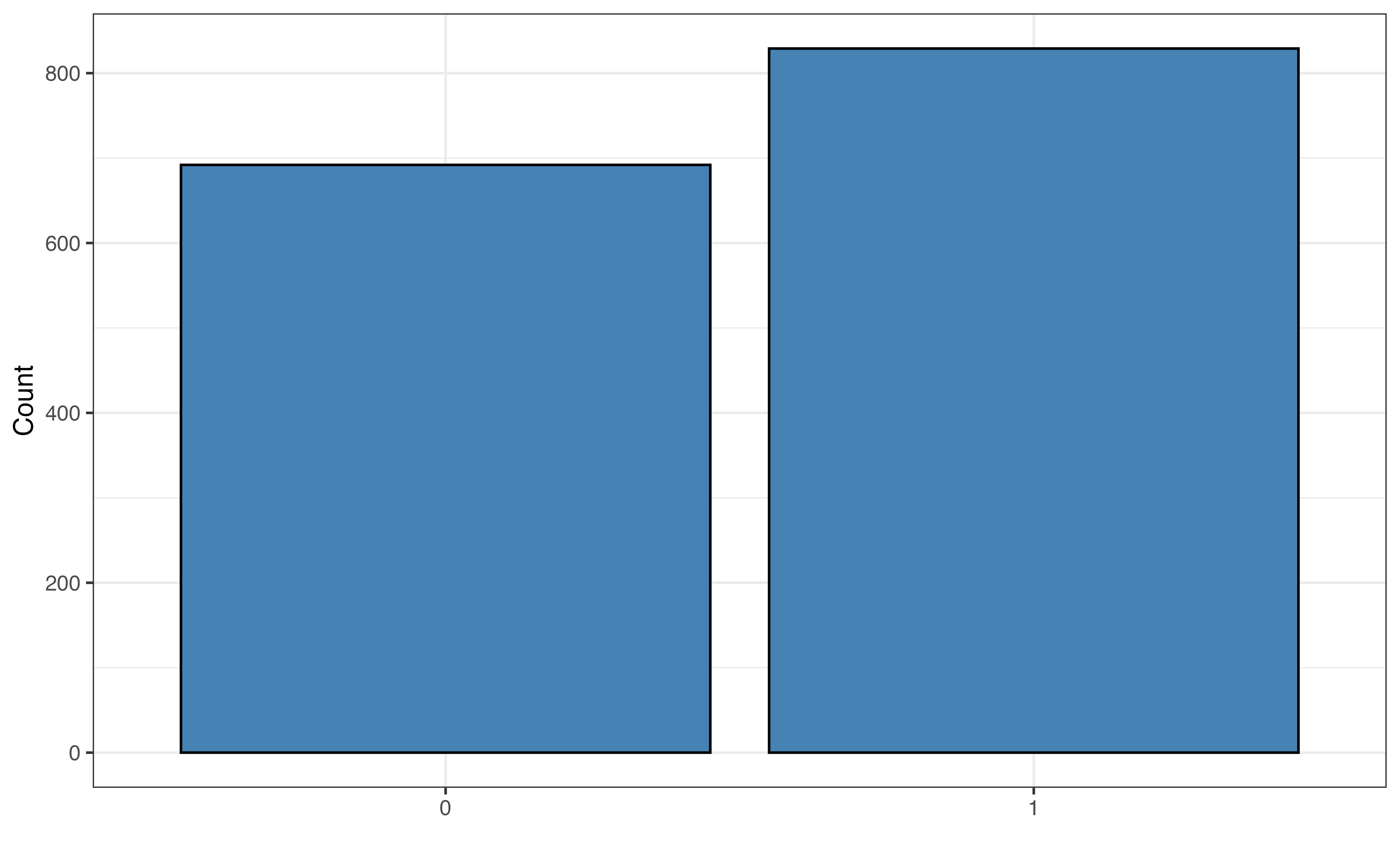
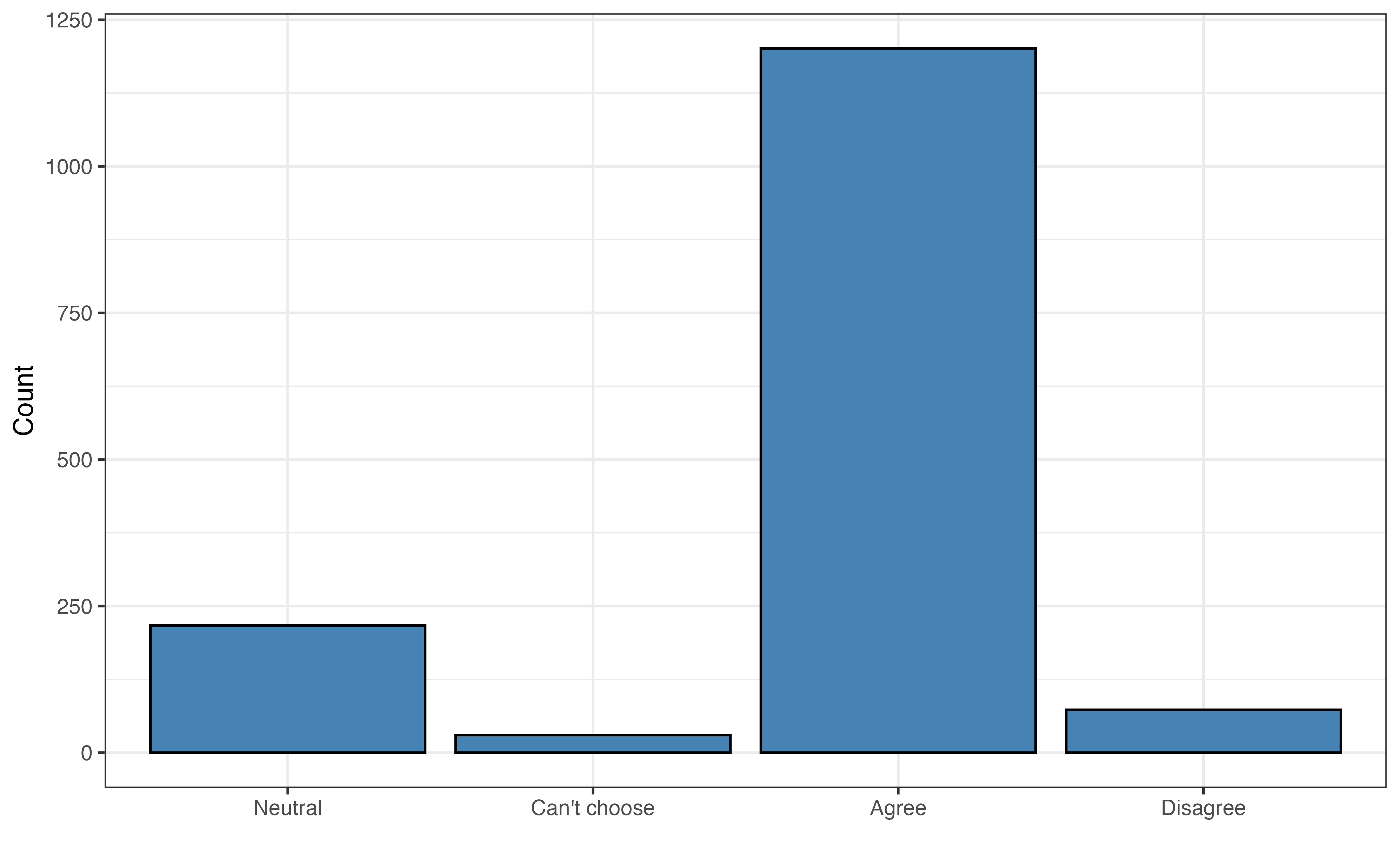
Figure 11.1 shows the distribution of the original responses to the survey question about comfort with driverless cars and aidrive_comfort, the binary variable we will use in the analysis. In practice, categorical variables may have many categories, so we can aggregate categories to simplify the variable based on the analysis question. We saw an example of this in Section 3.4.1 when we looked at the variable season created from month. By simplifying the variable, we change the scope of the variable from a rating of the level of comfort an individual has with driverless cars to whether or not an individual has comfort with driverless cars. The latter aligns with the analysis objective and the modeling introduced in this chapter. Models for categorical response variables with three or more levels, such as the original survey responses, are introduced in Section 13.1.

In Figure 11.1 (b), we see about 45% of the respondents said they were “totally uncomfortable” with driverless cars and 55% reported some level of comfort with these cars. In the distribution of the original response variable in Figure 11.1 (a), among those who had at least some comfort, most had comfort levels of 5 or less. This detail could be important as we interpret the practical implications of the conclusions drawn from the analysis.

Table 11.1: Summary statistics for age

Variable	Mean	SD	Min	Q1	Median (Q2)	Q3	Max	Missing
age	50.4	17.6	18	36	49	65	89	0

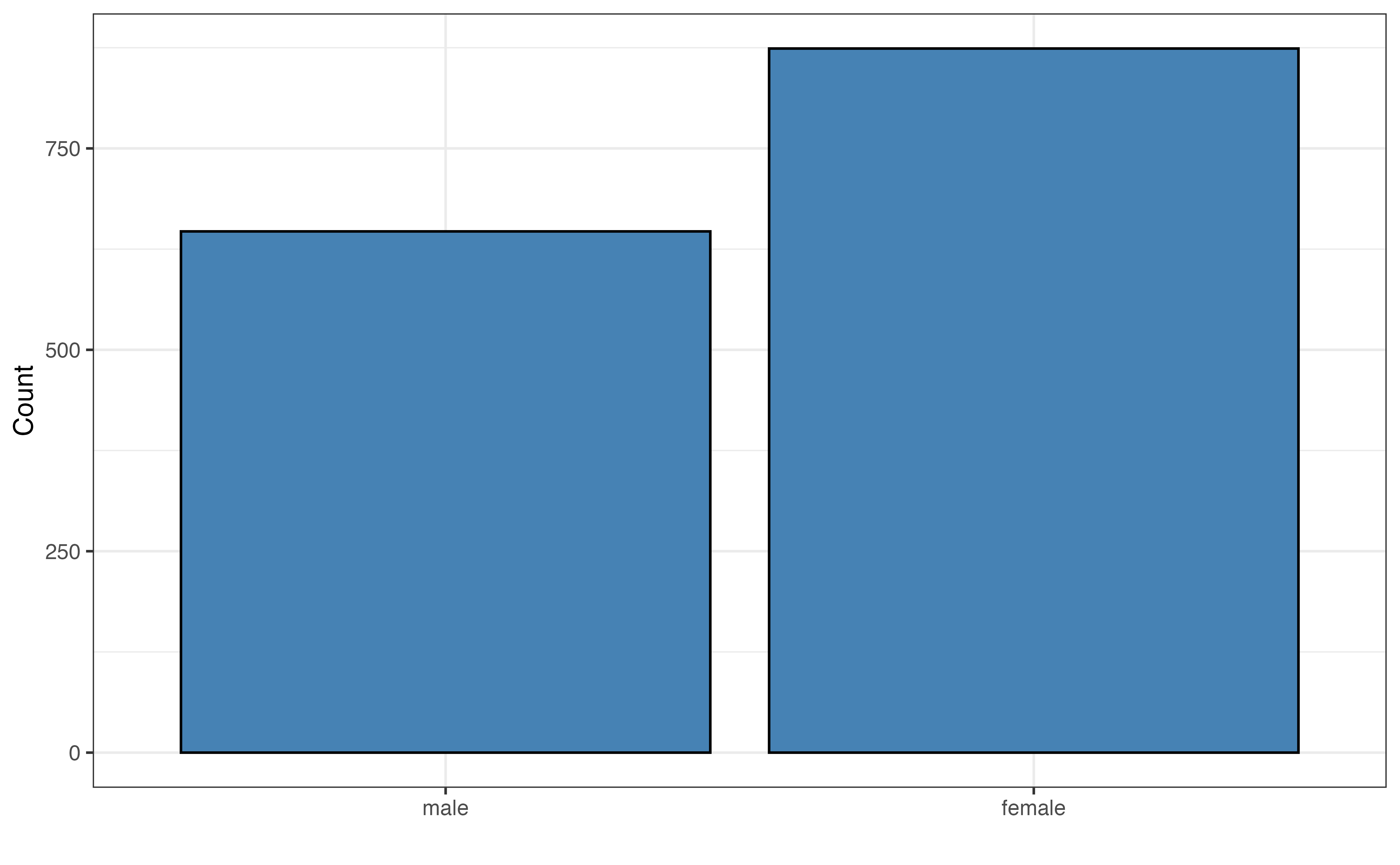
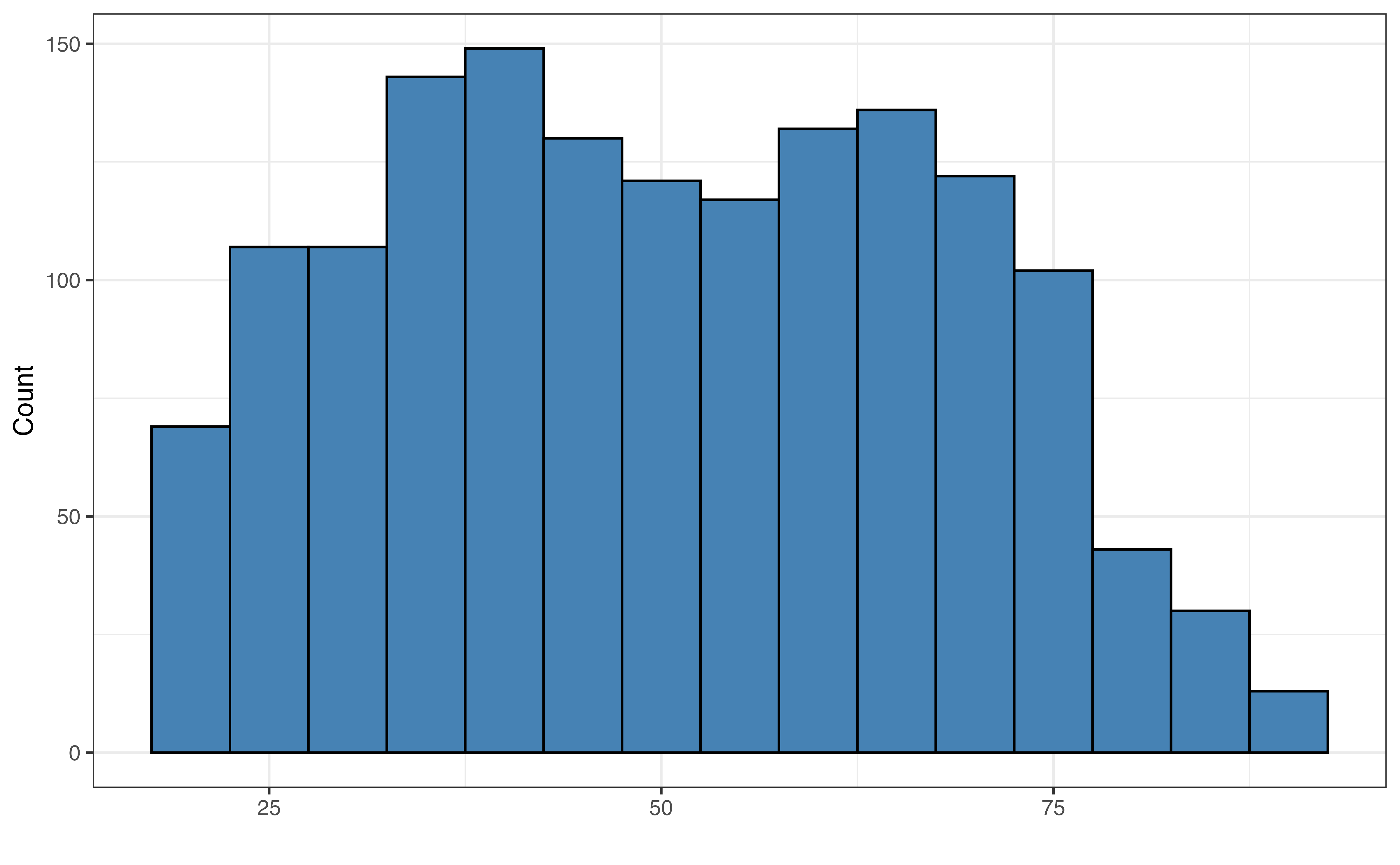
Figure 11.2 and Table 11.1 shows the univariate distributions of the predictor variables that will be used in this chapter. The exploratory data analysis for the other predictors is in Chapter 12 . The mean age in the data is about 50.4 and the median is 49 years old. The youngest respondents in the data set are 18 and the oldest are 89 years old. The standard deviation is about 17.645 years, so the data spans the general age range for adults in the United States.

We also observe from Figure 11.2 that the majority of the respondents (about 57 %) reported their sex as female, and a vast majority of respondents (about 79%) agree that technology is making life easier.

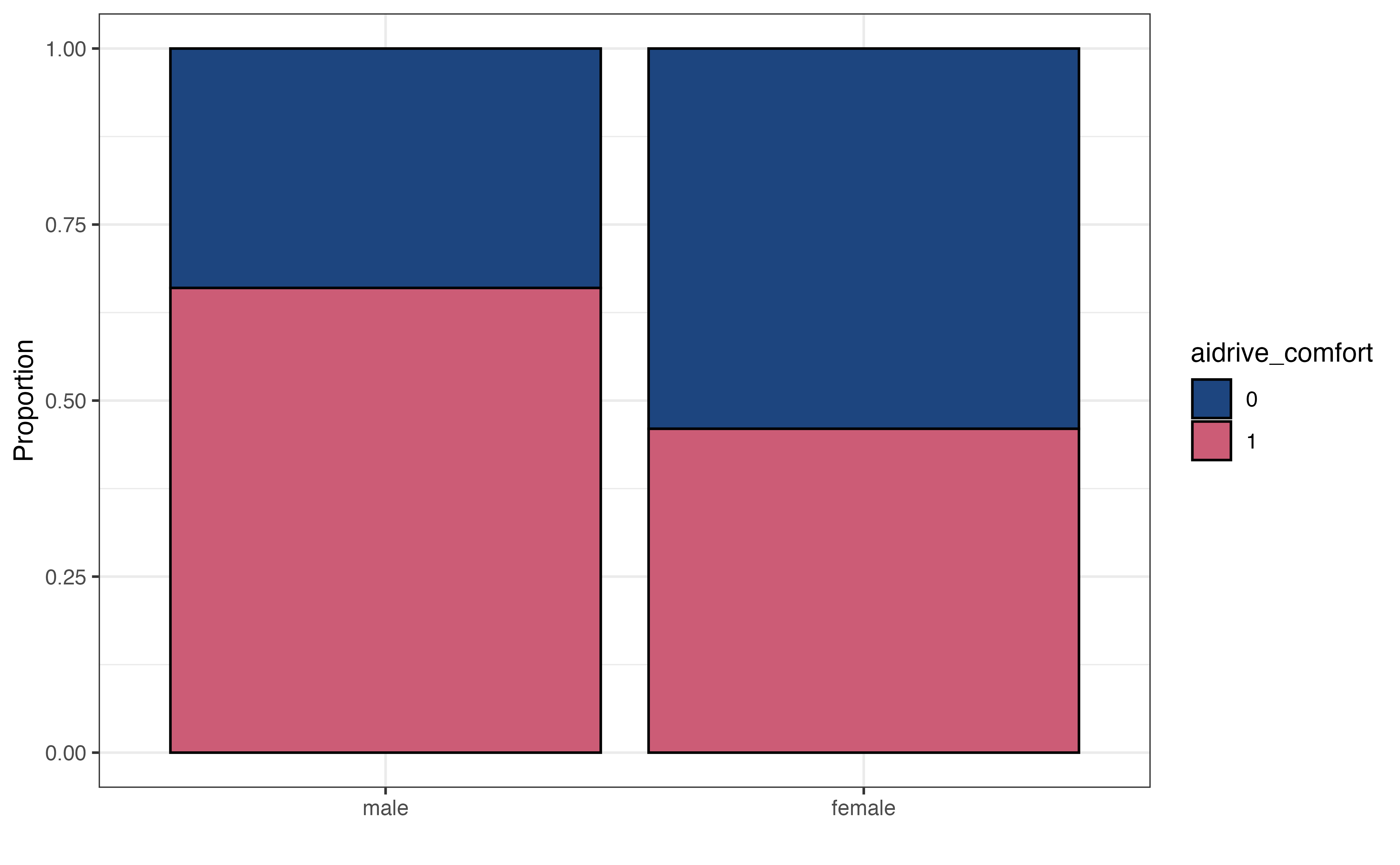
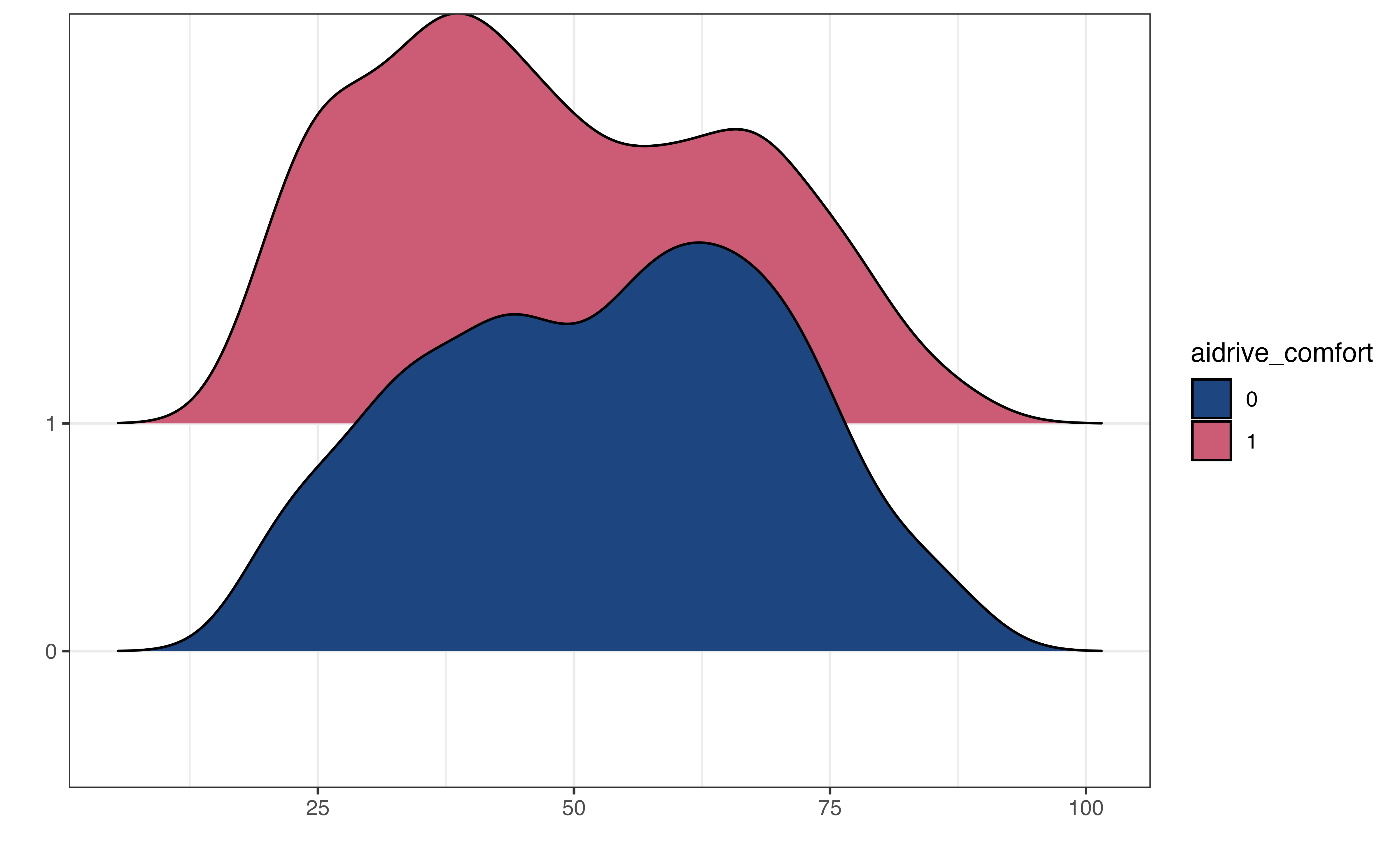
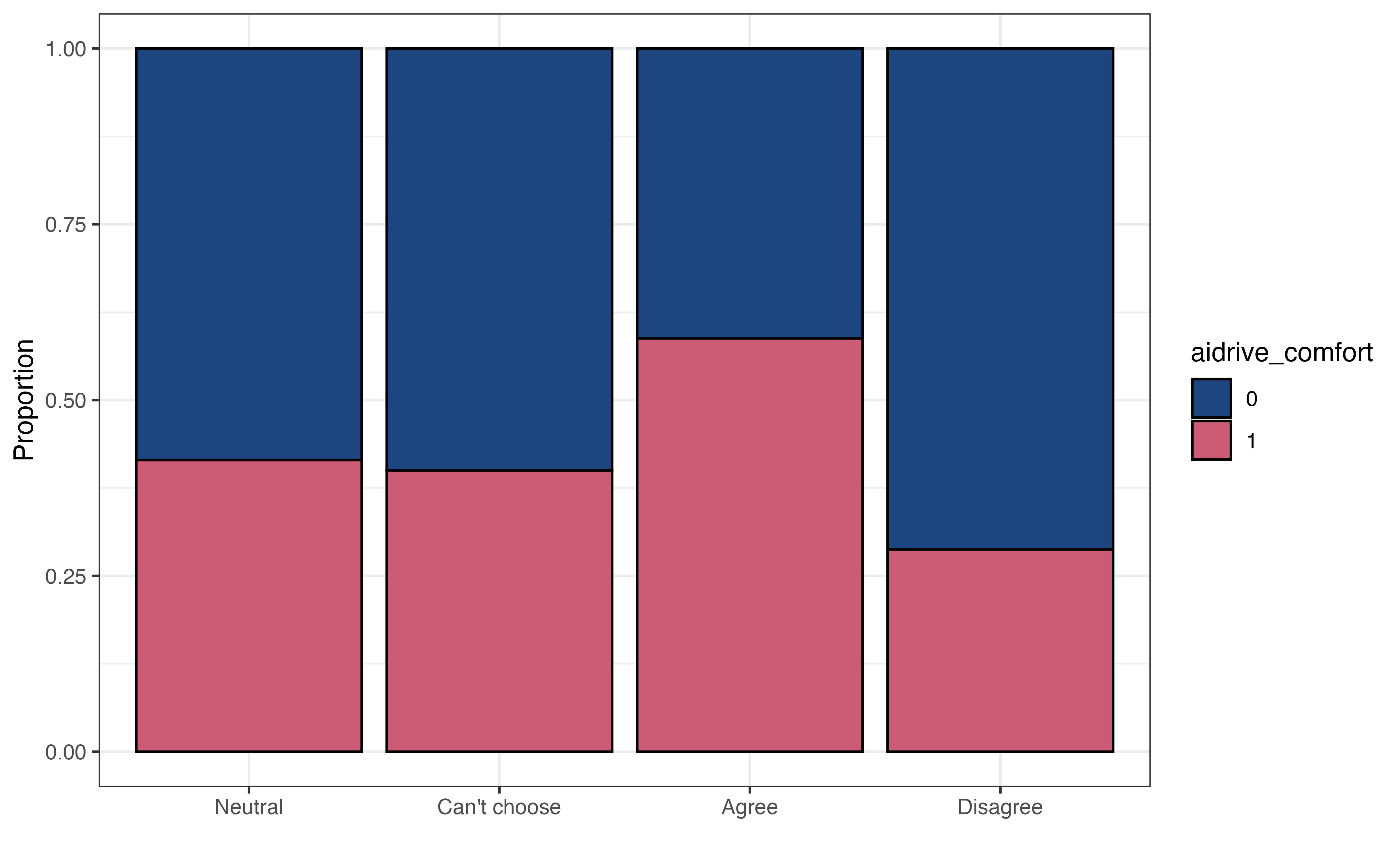
Figure 11.3 shows the relationship between the response and each of the predictor variables. Here we use a segmented bar plot to visualize the relationship between the categorical predictors, sex and tech_easy and the categorical response, aidrive_comfort. As we look at the segmented bar plot, we are evaluating distribution of the response variable is approximately equal for each category of the predictor (Section 3.5.3). Unequal proportions suggests some relationship between the response and predictor variable. In Figure 11.3, a higher proportion of males have comfort with driverless cars compared to the proportion of females. This indicates a potential relationship between sex and comfort with driverless cars. Figure 11.3 shows overlap in the distribution of age among those who have comfort with driverless cars versus those who do not, but the distribution among those who have comfort with driverless cars tends to skew younger. As with linear regression, however, we will use statistical inference Section 11.5 to determine if the data provide evidence that such relationships exist.

Based on Figure 11.3 , does there appear to be a relationship between opinions about whether technology makes life easier and comfort with driverless cars? Explain.¹

Now we use multivariate exploratory data analysis to explore potential interaction effects. Recall from Section 7.7 that an interaction effect occurs when the relationship between the response variable and a predictor differs based on values of the another predictor. We are often interested in interactions that include at least one categorical predictor, because we are interested how relationships might differ for subgroups in the sample.

(a) `aidrive` versus `age` faceted by `tech_easy`

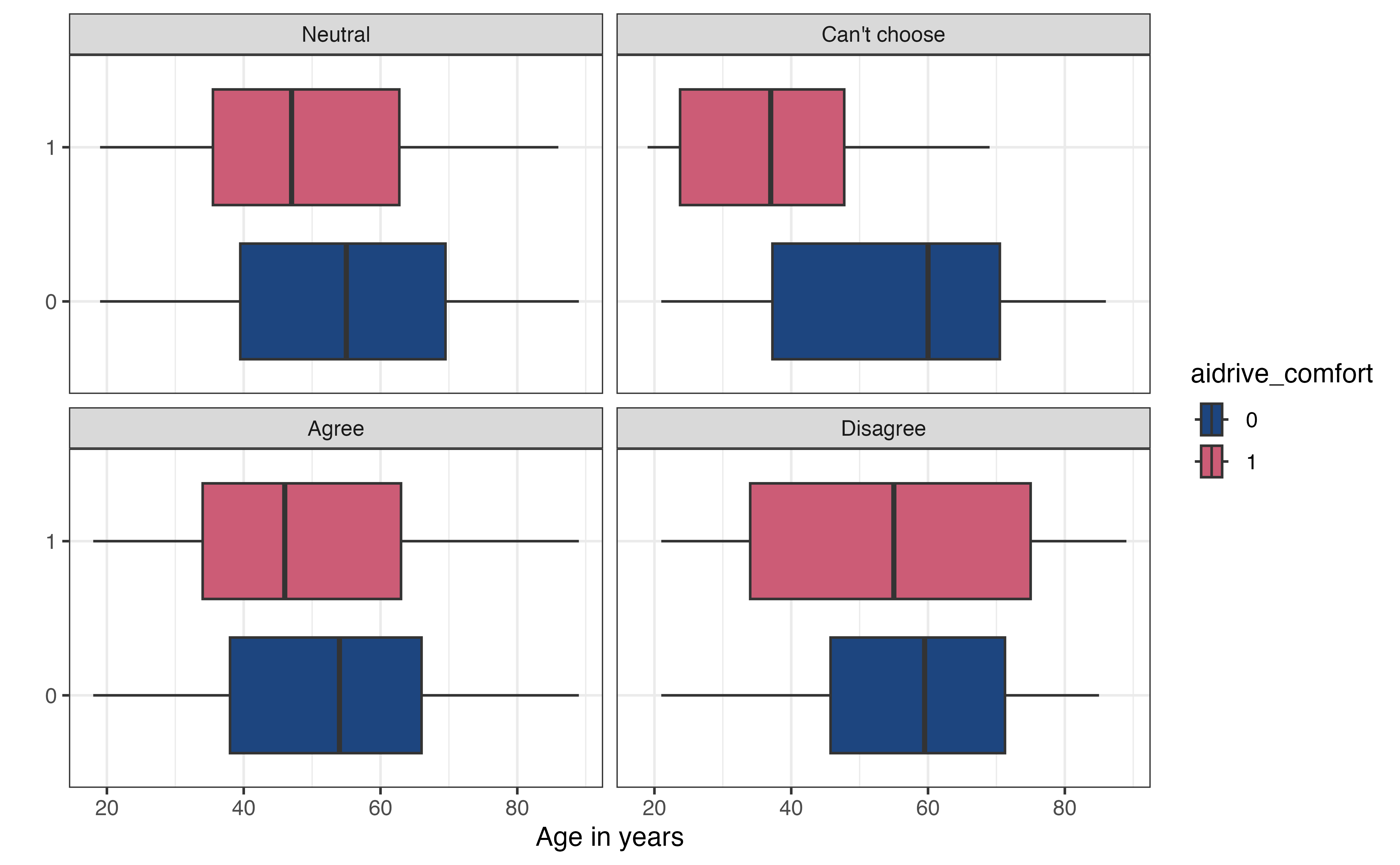
Figure 11.4 (a) is the relationship between age and aidrive_comfort faceted by the categories of tech_easy. As we look at the four sets of boxplots, we observe whether the relationship of the boxplots is the same for each level of tech_easy. If so, this indicates the relationship between age and aidrive_comfort is the same regardless of the value of tech_easy. In Figure 11.4 (a), the relationship in the distributions of age between those who have comfort with driverless cars versus those who don’t looks similar for the categories “Neutral”, “Agree”, and “Disagree”. The boxes largely overlap and the median age is approximately the same between the two groups of aidrive_comfort. The relationship does appear to be different among those in the “Can’t choose” category, as the median age among those who are not comfortable with driverless cars is higher than those who are comfortable.

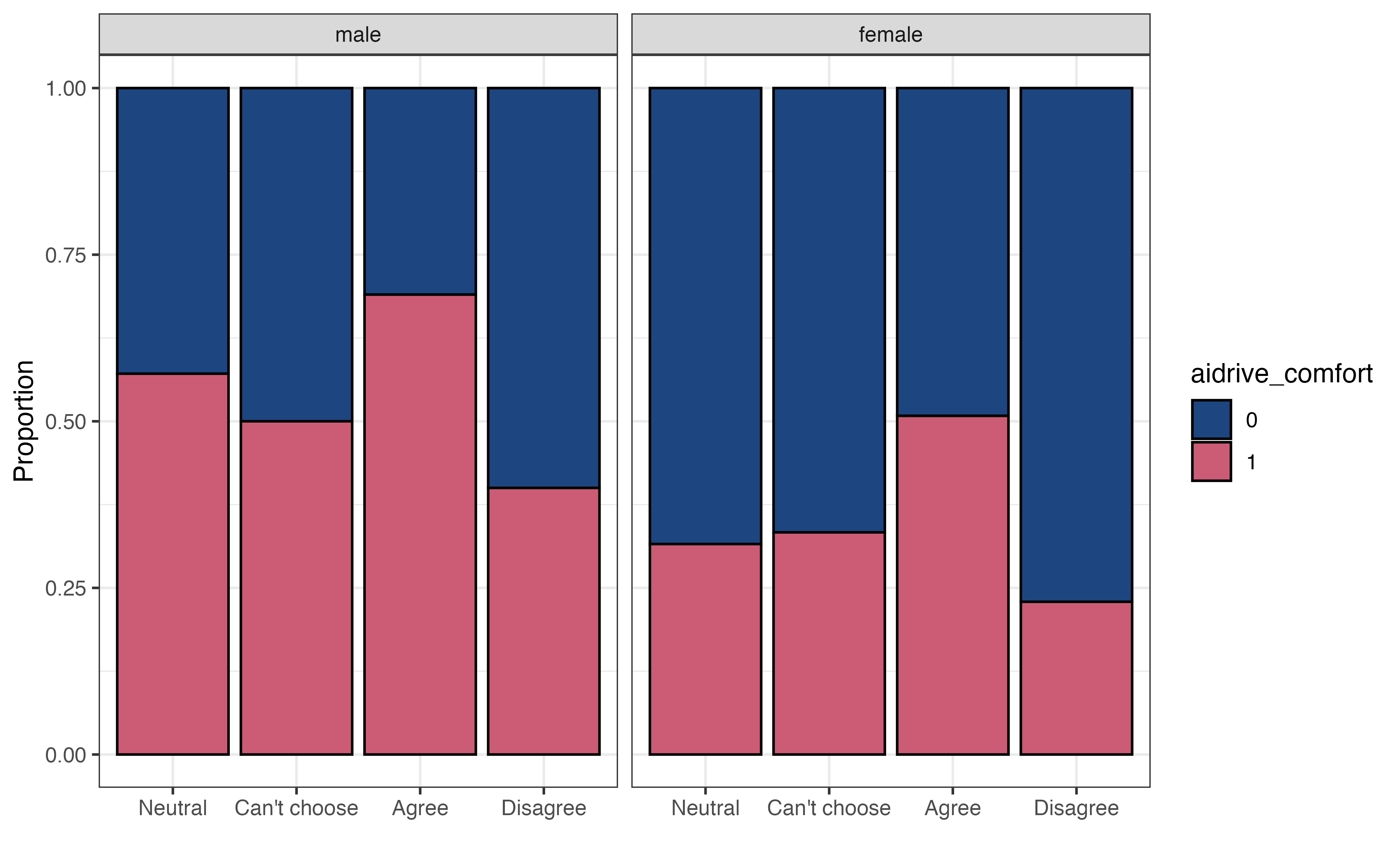
Figure 11.4 (b) is a plot to explore the interaction between two categorical predictors sex and tech_easy. Similar as before, we are examining whether the relationship between tech_easy and aidrive_comfort differs based on sex. We are not looking to see whether the proportions are equal between the two groups but are instead looking to see whether the proportions are approximately equal relative to one another within each category of sex.

Using this as the criteria, the relationship between tech_easy and aidrive_comfort looks approximately equal for the categories of sex. Therefore, the data do not show evidence of an interaction between tech_easy and sex. We do note that in general, the proportion of males comfortable with driverless cars within each group of tech_easy is higher than the corresponding groups for females. This is expected, given what we observed in the bivariate EDA in Figure 11.3.

11.2 Probability / odds/ odds ratio

11.2.1 Probability and odds

Before moving to modeling, let’s take some time to focus on the response variable. The response variable $Y$ is categorical and takes values “0” or “1”. The response $Y = 1$ indicates an observation takes the outcome of interest, and $Y = 0$ indicates an observation does not take that outcome. Sometimes $Y = 1$ and $Y = 0$ are called “success” and “failure”, respectively. Note, however, that a “success” just means it is the outcome we are interested in studying, not necessarily what would be considered a “success” in practice.

The probability $Y = 1$ , denoted $P r (Y = 1)$ , is a measure of the chance that the event $Y = 1$ occurs. Probabilities take values between 0 and 1, with 0 indicating an event is impossible and never occurs, and 1 indicating that an event always occurs. The odds $Y = 1$ are the ratio of the probability $Y = 1$ occurs versus the probability $Y = 0$ occurs. This is computed as

$\begin{matrix} (11.1) & odds(Y = 1) = \frac{P r (Y = 1)}{P r (Y = 0)} = \frac{P r (Y = 1)}{1 - P r (Y = 1)} \end{matrix}$

Note that the odds that $Y = 0$ are equal to $1 / odds (Y = 1)$ .

Table 11.2: Frequency, probability, and odds of aidrive_comfort

aidrive_comfort	n	probability	odds
0	692	0.455	0.835
1	829	0.545	1.198

Table 11.2 shows the probabilities an odds for the response variable aidrive_comfort. In the data from 1521 respondents, the probability (chance) a randomly selected respondent is comfortable with driverless cars is 0.545. This may also be phrased as there is a 54.5 % chance a randomly selected respondent is comfortable with driverless cars. The odds a randomly selected respondent is comfortable with driverless cars are 1.198. This means that a randomly selected respondent is 1.198 times more likely to be comfortable with driverless cars than not be.

Show how the following values are computed:

$P r (aidrive_comfort = 1) =$ 0.545
$odds (aidrive_comfort = 1) =$ 1.198 ²

11.2.2 Odds ratio

We are most interested in understanding the relationship between comfort with driverless cars and other factors about the respondents. Table 11.3 is a two-way table of the relationship between aidrive_comfort and tech_easy. Now we can not only answer questions regarding opinions about comfort with driverless cars overall but can also see how these opinions on comfort may differ based on respondent’s opinion about whether technology makes life easier.

Table 11.3: Two-way table of aidrive_comfort (columns) versus tech_easy (rows)

Tech Easy	0	1
Neutral	127	90
Can’t choose	18	12
Agree	495	706
Disagree	52	21

Each cell in the table is the number of observations that take the values indicated by the row and column. For example, there are 90 respondents in the data whose observed data are tech_easy = "Neutral" and aidrive_comfort = "1". We can use this table to ask how the probability of being comfortable with driverless cars differs based on opinions about whether technology makes life easier. For example, we can compute the probability and the corresponding odds a randomly selected respondent is comfortable with driverless cars given they are neutral about whether technology makes life easier.

$\begin{matrix} (11.2) & \begin{array}{r} P r (Y = 1 | tech_easy = Neutral) = \frac{90}{127 + 90} \approx 0.415 \\ odds (Y = 1 | tech_easy = Neutral) = \frac{90}{127} = \frac{0.415}{1 - 0.415} \approx 0.709 \end{array} \end{matrix}$

$P r (Y = 1 | tech_easy = Neutral)$ is called a conditional probability, because it is the probability that a randomly selected respondent is comfortable with driverless cars conditioned on (given) they are neutral about whether technology makes life easier. Similarly, $odds (Y = 1 | tech_easy = Neutral)$ are conditional odds.

It may sound awkward to communicate results where the odds are less than 1. Because the odds are reciprocal, they are typically reported in terms of the odds being greater than 1. For example, an alternative way to present the odds from Equation 11.2 is

A randomly selected respondent who is neutral about technology making life easier is 1.41 times more likely to not be comfortable with driverless cars than be comfortable.

Compute the probability and corresponding odds of being comfortable with driverless cars among those who agree with the statement that technology makes life easier.³

From Table 11.3, the odds a respondent who is neutral about technology making life easier is comfortable with driverless cars are 0.709, and the odds a respondent who agrees technology makes life easier are 1.43. We quantify how the odds for these two groups compare using an odds ratio. An odds ratio is computed as the odds for one group divided the odds for another, as shown in Equation 11.3

$\begin{matrix} (11.3) & odds ratio = \frac{{odds}_{g r o u p 1}}{{odds}_{g r o u p 2}} \end{matrix}$

Let’s compute the odds ratio for those who agree that technology makes life easier versus those who are neutral.

$odds ratio = \frac{{odds}_{Agree}}{{odds}_{Neutral}} = \frac{1.43}{0.709} = 2.02$

This means that the odds a respondent who agrees technology makes life easier is comfortable with driverless cars are 2.02 times the odds a respondent who is neutral about technology is comfortable with driverless cars.

Compute the odds ratio of being comfortable with driverless cars for tech_easy = Agree versus teach_easy = Disagree. Interpret this value in the context of the data.⁴

11.3 From linear to logistic regression

The two-way table and odds ratios from the previous section helped us being to explore the relationship between comfort with driverless cars and opinion about whether technology makes life easier. Let’s build on this by fitting a model that can (1) help us quantify the relationship between variables, (2) explore the relationship between the response and multiple predictors variables, and (3) be used to make predictors and draw rigorous conclusions. Before diving into the details of this model’s we’ll take a moment to understand why we are introducing a new model for the relationship between aidrive_comfort versus the predictors rather than using the linear regression model we’ve seen up to this point.

Suppose we want to fit a model of the relationship between age and aidrive_comfort. Our first thought may be to use the linear regression model from Chapter 4 to model this relationship. In this case, the estimated model would be of the form

$\begin{matrix} (11.4) & \hat{aidrive_comfort} = {\hat{β}}_{0} + {\hat{β}}_{1} \times age \end{matrix}$

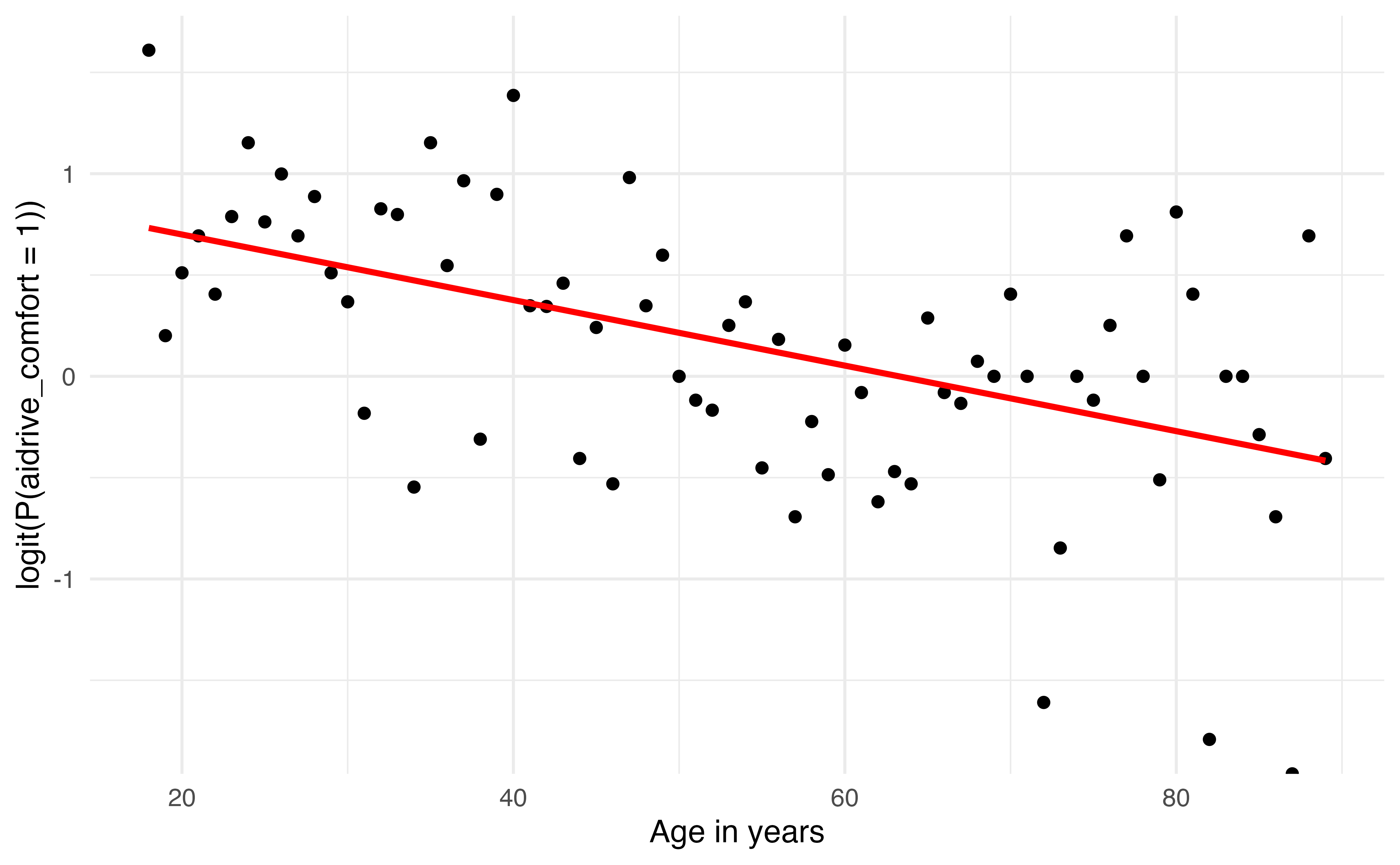
Figure 11.5: Linear regression model for `aidrive_comfort` versus `age`

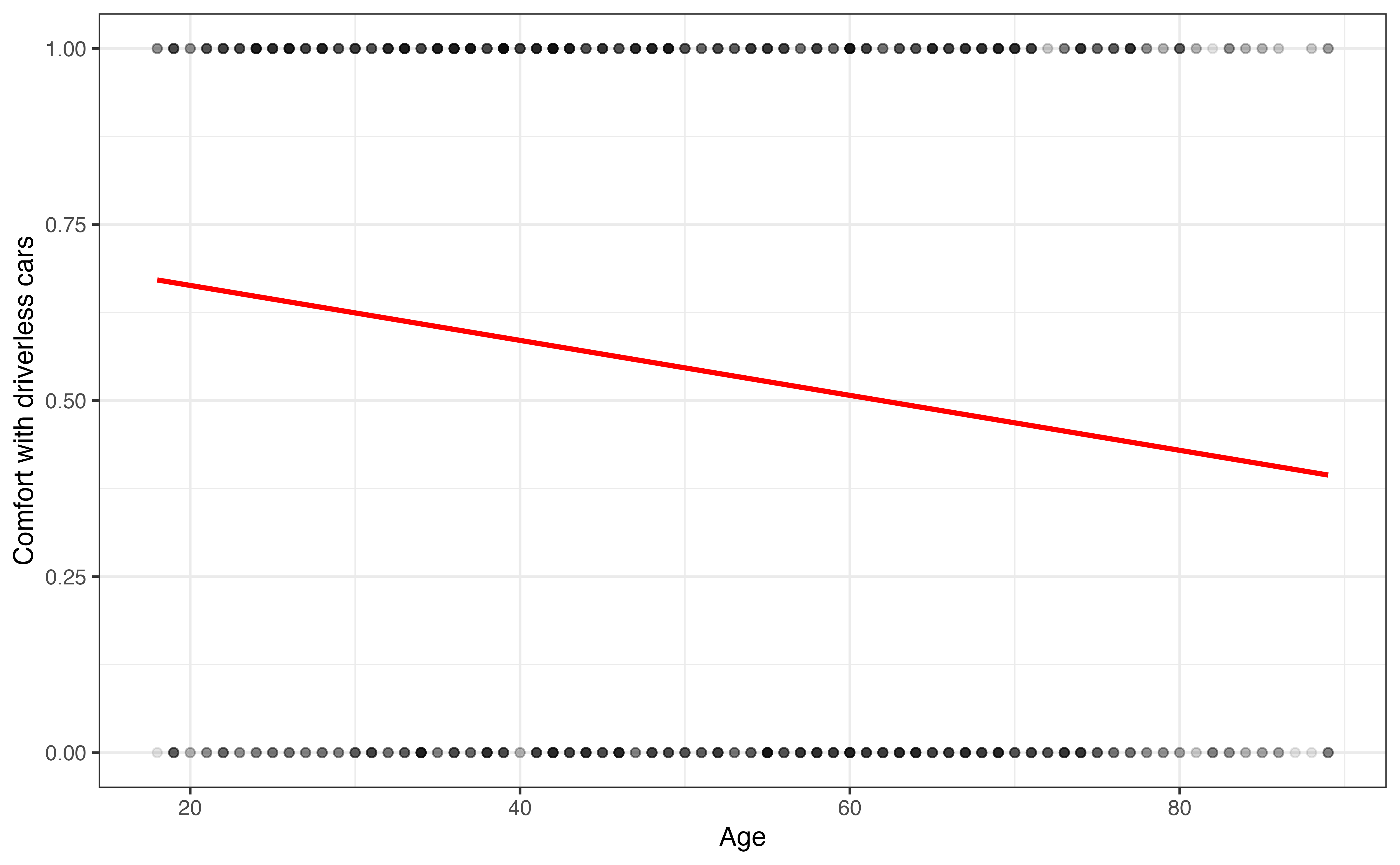
Figure 11.5 is a visualization of the linear regression model for the relationship between age and aidrive_comfort shown in Equation 11.4. Here we easily see the linear regression model represented by the red line is not a good fit for the data. In fact, it (almost) never produces predictions of 0 or 1, the observed values of the response. Recall that the linear regression model is estimated by minimizing the sum of squared residuals, $0 - {\hat{y}}_{i}$ or $1 - {\hat{y}}_{i}$ in this scenario. These residuals can be minimized by finding a model that produces estimates between 0 and 1, as shown in Figure 11.5, rather than trying to predict the actual observed values, 0 or 1.

Next, we might consider fitting a linear model such that the response variable is the $π = P r (Y = 1)$ , the probability of being comfortable with driverless cars. This estimated model takes the form

$\begin{matrix} (11.5) & \hat{π} = {\hat{β}}_{0} + {\hat{β}}_{1} \times age \end{matrix}$

Figure 11.6: Linear model for Pr(`aidrive_comfort = 1`) versus `age`

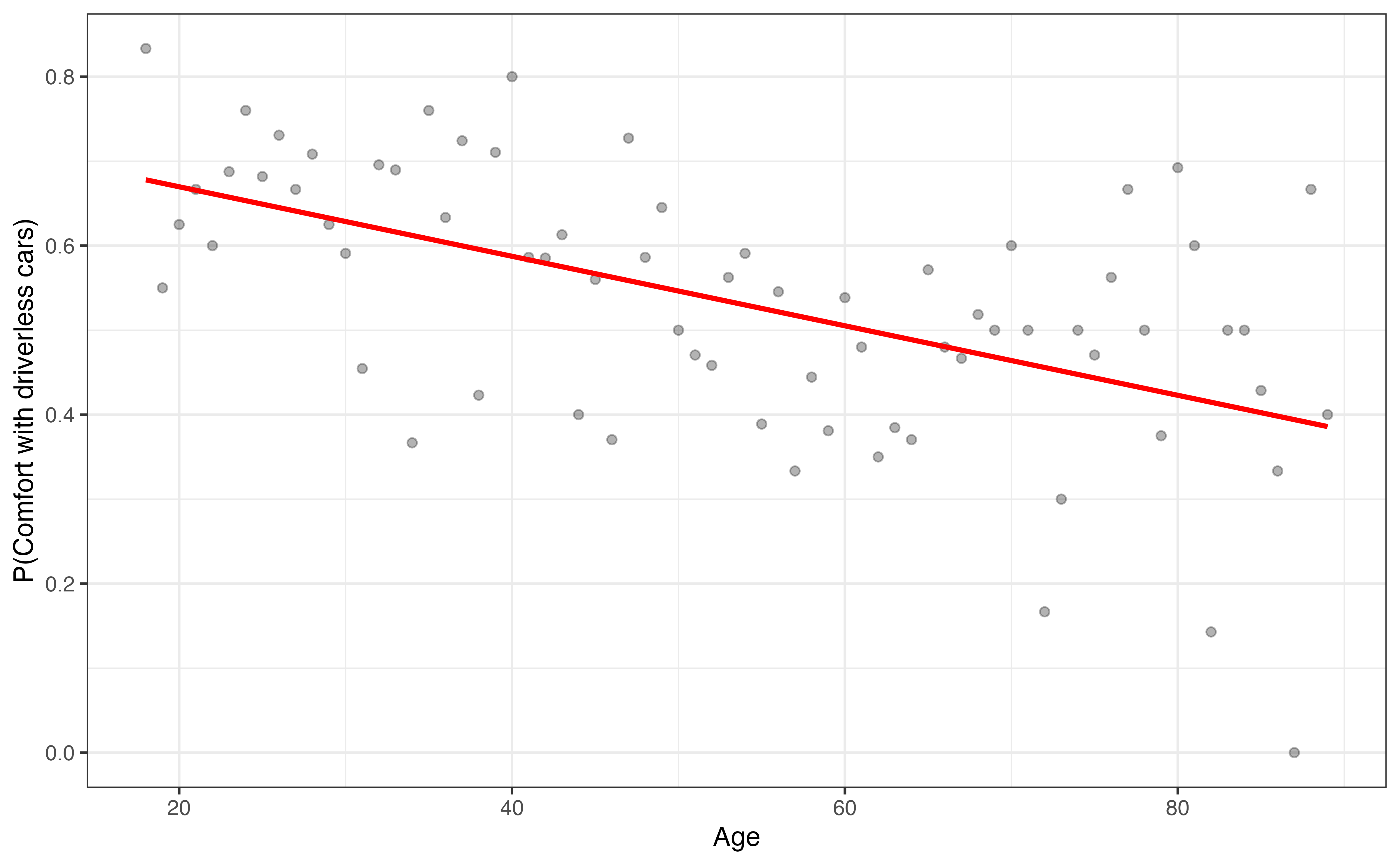
Figure 11.6 shows the relationship between age and the probability of being comfortable with driverless cars. This model seems to be a better fit for the data, as it generally captures the trend that younger respondents are more likely to be comfortable with driverless cars compared to older respondents. The primary issue with using the probability as the response variable is that probabilities are bounded between 0 and 1. Therefore, it is impossible to get values less than 0 or greater than 1 in practice, so we would want the same bounded constraints on our model particularly if we wish to use the model for prediction. We saw a similar issue in Chapter 10 with the values of valence in the Spotify data. We have the same issue when using the odds as the response variable, because the odds cannot be less than 0. Therefore, we need a model that not only captures the relationship between the response and predictor but also addresses the boundary constraint.

When there is a binary categorical response variable, we use a logistic regression model to model the relationship between the binary response and one or more predictor variables as in Equation B.1.

$\begin{matrix} (11.6) & \log (\frac{π}{1 - π}) = β_{0} + β_{1} x_{1} + \dots + β_{p} x_{p} \end{matrix}$

where $π = P r (Y = 1)$ and $\log (\frac{π}{1 - π})$ is the logit transformation, also called the “log odds”. The log odds can take any value $- \infty$ to $\infty$ , so it does not have the boundary constraints of the probability and odds. The log odds output from Equation B.1 can be transformed back to the odds and probabilities, and we will the probabilities to assign each observation to a predicted class aidrive_comfort = 0 or aidrive_comfort = 1. We’ll discuss this more in Chapter 12.

Figure 11.7: Output from logistic regression model of `aidrive_comfort` versus `age`

Figure 11.7 shows the output of the logistic regression model of aidrive_comfort versus age. Here, we see the logit is not bounded as the probability or odds.

Equation B.1 is the statistical model for logistic regression. The statistical model does not have the error term $ϵ$ as we’ve seen in the statistical model for linear regression in Equation 7.3. Recall from Section 7.2 that the error term $ϵ$ is the difference between the observed response $Y$ and the expected value produced by the model $β_{0} + β_{1} x_{1} + \dots + β_{p} x_{p}$ . Thus, we produce predictions for the response variable directly when doing linear regression.

In contrast, the output of the logistic regression model are the log odds that $y = 1$ , not the actual observed values $y_{i} = 0$ or $y_{i} = 1$ . Thus, there is no error term in the statistical model for logistic regression, because we do not predict the value of the response directly and thus do not have the same notion of the difference between the observed and predicted response.

11.4 Interpreting model coefficients

In Section 7.3, we showed that the model coefficients for linear regression are estimated by the least-squares method, finding the values of the coefficients that minimizes the sum of squared residuals. There is no error term in the logistic regression model (see ?eq-logistic-model-2), so we cannot use least-squares in this case. The model coefficients for logistic regression are estimated using maximum likelihood estimation. Recall from Section 10.2 that the likelihood is a function that quantifies how likely the observed data are to have occurred given a combination of coefficients. Thus, maximum likelihood estimation is used to find the combination of coefficients that makes the observed data the most likely to have occurred, i.e., that maximizes the value of the likelihood function. The mathematical details for estimating logistic regression coefficients using maximum likelihood estimation are available in Section B.2.

11.4.1 Predictor in simple logistic regression

In Section 11.2, we computed values from a two-way table to understand the relationship between opinions about whether technology makes life easier and comfort with driverless cars. Now we will use a logistic regression model to quantify the relationship.

Table 11.4: Logistic regression model for aidrive_comfort versus tech_easy

term	estimate	std.error	statistic	p.value
(Intercept)	-0.344	0.138	-2.499	0.012
tech_easyCan’t choose	-0.061	0.397	-0.154	0.878
tech_easyAgree	0.699	0.150	4.671	0.000
tech_easyDisagree	-0.562	0.293	-1.919	0.055

Equation 11.7 is the equation from the model output in Table 11.4.

$\begin{matrix} (11.7) & \begin{array}{r} \log (\frac{\hat{π}}{1 - \hat{π}}) = - 0.344 + - 0.061 \times Can’t choose + 0.699 \times Agree - 0.562 \times Disagree \end{array} \end{matrix}$

where $\hat{π}$ is the predicted probability a respondent is comfortable with driverless cars.

What is the baseline level for tech_easy? ⁵

The intercept, -0.344, is the estimated log odds for respondents in the baseline group, Neutral. Similar to interpretations in Section 9.2, though we do calculations using the logit, we write interpretations in terms of the odds, so they are more clearly understood by the reader. To transform from logit to odds, we exponentiate both sides of the model equation. Equation 11.8 shows the equation from Table 11.4 in terms of the odds of being comfortable with driverless cars.

$\begin{matrix} (11.8) & \begin{array}{r} \frac{\hat{π}}{1 - \hat{π}} = e^{- 0.344} \times e^{- 0.061 \times Can’t choose} \times e^{0.699 \times Agree} \times e^{- 0.562 \times Disagree} \end{array} \end{matrix}$

From Equation 11.8, we see that the estimated odds a respondent who is neutral about whether technology makes life easier is comfortable with driverless cars is 0.709 ( $e^{- 0.344}$ ). This equals the odds that was computed from the two-way table in Equation 11.2.

The following two rules were used to go from Equation 11.7 to Equation 11.8

$e^{\log (a)} = a$
$e^{a + b} = e^{a} e^{b}$

Now let’s look at the coefficient for Agree, 0.699. Putting together what know about the response variable with what we’ve learned about interpreting coefficients for categorical predictors in Section 7.4.2, this estimated coefficient means the following:

The log odds a respondent who agrees technology makes life easier is comfortable with driverless cars are expected to be 0.699 higher than the log odds of a respondent who is neutral about whether technology makes life easier.

From Equation 11.8, the coefficient for Agree is $e^{0.699} \approx 2.012$ . This means the following:

The odds a respondent who agrees technology makes life easier is comfortable with driverless cars are expected to be 2.012 ( $e^{0.699}$ ) times the odds of a respondent who is neutral about whether technology makes life easier.

The value 2.012 is equal to the odds ratio of aidrive_comfort = 1 for tech_easy = Agree versus tech_easy = Neutral. It is the same (give or take rounding) as the odds ratio we computed from Table 11.3. This tells us something important about the relationship between the odds ratio and model coefficients in a logistic regression model. When we fit a simple logistic regression model with one categorical predictor $X$ such that $β_{k}$ is the coefficient corresponding to the $k^{t h}$ level of $X$ , then $e^{β_{k}}$ is the odds ratio between the $k^{t h}$ level and the baseline level.

11.4.2 Categorical predictors

Now, we will fit a multiple logistic regression model and use age along with tech_easy as predictors aidrive_comfort.

Table 11.5: Logistic regression model for aidrive_comfort versus age and tech_easy

term	estimate	std.error	statistic	p.value
(Intercept)	0.420	0.208	2.020	0.043
tech_easyCan’t choose	-0.118	0.402	-0.294	0.769
tech_easyAgree	0.678	0.151	4.487	0.000
tech_easyDisagree	-0.499	0.295	-1.690	0.091
age	-0.015	0.003	-4.902	0.000

Now that we have multiple predictors in Table 11.5, the intercept is the predicted log odds of being comfortable with driverless cars for those who are neutral about technology making life easier and who are 0 years old. It would be impossible for a respondent to be 0 years old, so while the intercept is necessary to obtain the best fit model, its interpretation is not meaningful in practice. As with linear regression, we could use the centered values of age in the model if we wish to have an interpretable intercept.

The coefficient for Agree in this model is 0.678. It is but not equal to the coefficient for Agree in the previous model, because now the coefficient is computed after adjusting for age. The interpretation is similar as before, taking into account the fact that age is also in the model.

The log odds a respondent who agrees technology makes life easier is comfortable with driverless cars are expected to be 0.678 higher than the log odds of a respondent who is neutral about whether technology makes life easier, holding age constant.

To write the interpretation in terms of the odds, we need to exponentiate both sides of the model equation as in the previous section. Equation 11.9 shows the relationship between opinions about technology, age, and the odds of being comfortable with driverless cars.

$\begin{matrix} (11.9) & \begin{array}{r} \frac{\hat{π}}{1 - \hat{π}} = e^{0.420} \times e^{- 0.118 \times Can’t choose} \times e^{0.678 \times Agree} \times e^{- 0.499 \times Disagree} \times e^{- 0.015 \times age} \end{array} \end{matrix}$

where $\hat{π}$ is the predicted probability a respondent is comfortable with driverless cars.

Based on Equation 11.9, the interpretation of the Agree in terms of the odds is the following:

The odds a respondent who agrees technology makes life easier is comfortable with driverless cars are expected to be 1.970 ( $e^{0.678}$ ) times the odds of a respondent who is neutral about whether technology makes life easier, holding age constant.

The value 1.970 ( $e^{0.678}$ ) is the odds ratio of comfort with driverless cars between those who agree technology makes life easier and those who are neutral, after adjusting for age. When there are multiple predictor variables in the logistic regression model, $e^{β_{j}}$ where $β_{j}$ is the coefficient for the predictor is called the adjusted odds ratio (AOR).

Use the model from Table 11.5. Assume age is held constant.

Interpret the coefficient of Disagree in terms of the log odds of being comfortable with driverless cars.
Interpret the coefficient of Disagree in terms of the odds of being comfortable with driverless cars.⁶

11.4.3 Quantitative predictors

Similar to categorical predictors, we can use what we learned about interpreting quantitative predictors in linear regression models in Section 7.4.1 as a starting point for interpretations for logistic regression. Let’s look at the interpretation of the coefficient for age from the model in Table 11.5. The coefficient is the expected change in the response when the predictor increases by one unit . Given this, the interpretation for age in terms of the log odds is the following:

For each additional year increase in age, the log odds a respondent is comfortable with driverless cars are expected to decrease by 0.015, holding opinions about technology constant.

Let’s take a moment to show this interpretation mathematically by comparing the log odds between age and age + 1, where age+1 represents the one unit increase in age. The interpretations are written holding opinions about technology constant, so we can ignore this predictor when doing these calculations. We’ll also ignore the intercept, because it is also the same regardless of the value of age. Let $log odds (comfort | age)$ be the log odds given some value age and $log odds (comfort | age + 1)$ be the log odds given the value age + 1.

Then, the change in the log odds is

$\begin{matrix} (11.10) & \begin{aligned} log odds (comfort | age + 1) - log odds (comfort | age) & = - 0.015 \times (age + 1) - (- 0.015 \times age) \\ = - 0.015 (age + 1 - age) \\ = - 0.015 \end{aligned} \end{matrix}$

From Equation 11.10, $log odds (comfort | age + 1) = log odds (comfort | age) - 0.015$ .

Now we’ll interpret the coefficient of age in terms of the odds. Based on Equation 11.9, the interpretation of age in terms of the odds of being comfortable with driverless cars is the following:

For each additional year increase in age, the odds a respondent is comfortable with driverless cars are expected to multiply by 0.985 ( $e^{- 0.015}$ ), holding opinions about technology constant.

$\log (a) + \log (b) = \log (a b)$

$\log (a) - \log (b) = \log (\frac{a}{b})$

We can show the interpretation mathematically starting with the result from Equation 11.10.

$\begin{matrix} (11.11) & \begin{aligned} log odds (comfort | age + 1) - log odds (comfort | age) & = - 0.015 \\ \Rightarrow \log (\frac{odds (comfort | age + 1)}{odds (comfort | age)}) & = - 0.015 \\ * exponetiate both sides * \\ \Rightarrow \frac{odds (comfort | age + 1)}{odds (comfort | age)} & = e^{- 0.015} \end{aligned} \end{matrix}$

From Equation 11.11, $odds (comfort | age + 1) = e^{- 0.015} \times odds (comfort | age)$ . The value $\frac{odds (comfort | age + 1)}{odds (comfort | age)}$ is the odds ratio of being comfortable with driverless cars between age versus age + 1. Thus, given $β_{j}$ is the coefficient for a quantitative predictor $X_{j}$ , the value $e^{β_{j}}$ is the (adjusted) odds ratio between $X_{j} + 1$ and $X_{j}$ .

Use the model in Table 11.5. Assume opinions about technology are held constant.

How are the log odds of being comfortable with driverless cars expected to change when age increases by 5 years?
How are the odds of being comfortable with driverless cars expected to change when age increases by 5 years? ⁷

11.5 Inference for a coefficient $β_{j}$

Inference for coefficients in logistic regression is very similar to inference in linear regression, introduced in Chapter 5 and Chapter 8. We will use these chapters as the foundation, discuss how they apply to logistic regression, and show ways in which inference for logistic regression differs. We refer the reader to the chapters on inference for linear regression for an introduction to statistical inference more generally.

11.5.1 Simulation-based inference

We can use simulation-based inference to draw conclusions about the model coefficients in logistic regression. The process for constructing bootstrap confidence intervals and using permutation sampling for hypothesis tests are the same as in linear regression, with the difference being the type of model that is fit. Here we will show how they apply to logistic regression.

Permutation tests

Hypothesis tests is used to test a claim about a population parameter. In the case of logistic regression, we use hypothesis tests to evaluate whether there is evidence of a relationship between a given predictor and the log odds of the response variable. The hypotheses to test whether there is a relationship between predictor $X_{j}$ and the response, after adjusting for the other predictors are in Equation 11.12.

$\begin{matrix} (11.12) & \begin{aligned} H_{0} : β_{j} = 0 - There is no relationship between X_{j} and the response \\ H_{a} : β_{j} \neq 0 - There is a relationship between X_{j} and the response \end{aligned} \end{matrix}$

The hypothesis test is conducted assuming the null hypothesis is true. When doing simulation-based inference, we use permutation sampling to generate the null distribution under this assumption. The process for permutation sampling is the same for logistic regression as with linear regression in Section 5.6. The values of the predictor of interest $X_{j}$ are permuted, such that the values are randomly assigned to each observation. There is no relationship between the permuted values of $X_{j}$ and the response variable. The logistic model is fit to each permuted sample, and the estimated coefficients ${\hat{β}}_{j}$ from the permuted samples make up the null distribution. The null distribution is used to compute the p-value and draw a conclusion about the hypotheses.

We’ll use a permutation test to evaluate whether there is evidence of a relationship between age and aidrive_comfort , after adjusting for tech_easy.

$\begin{array}{r} H_{0} : β_{age} = 0 vs β_{age} \neq 0 \end{array}$

The original value and five permutations of age for the first respondent are shown Table 11.6.

Table 11.6: Five permutations of age for Respondent 1

	aidrive_comfort	tech_easy	age
Original Sample	1	Agree	33
Permutation 1	1	Agree	31
Permutation 2	1	Agree	34
Permutation 3	1	Agree	69
Permutation 4	1	Agree	48
Permutation 5	1	Agree	80

Table 11.6 illustrates permutation sampling for one respondent. For each permutation, the value of aidrive_comfort and tech_easy are the same, and the values of age are randomly shuffled.

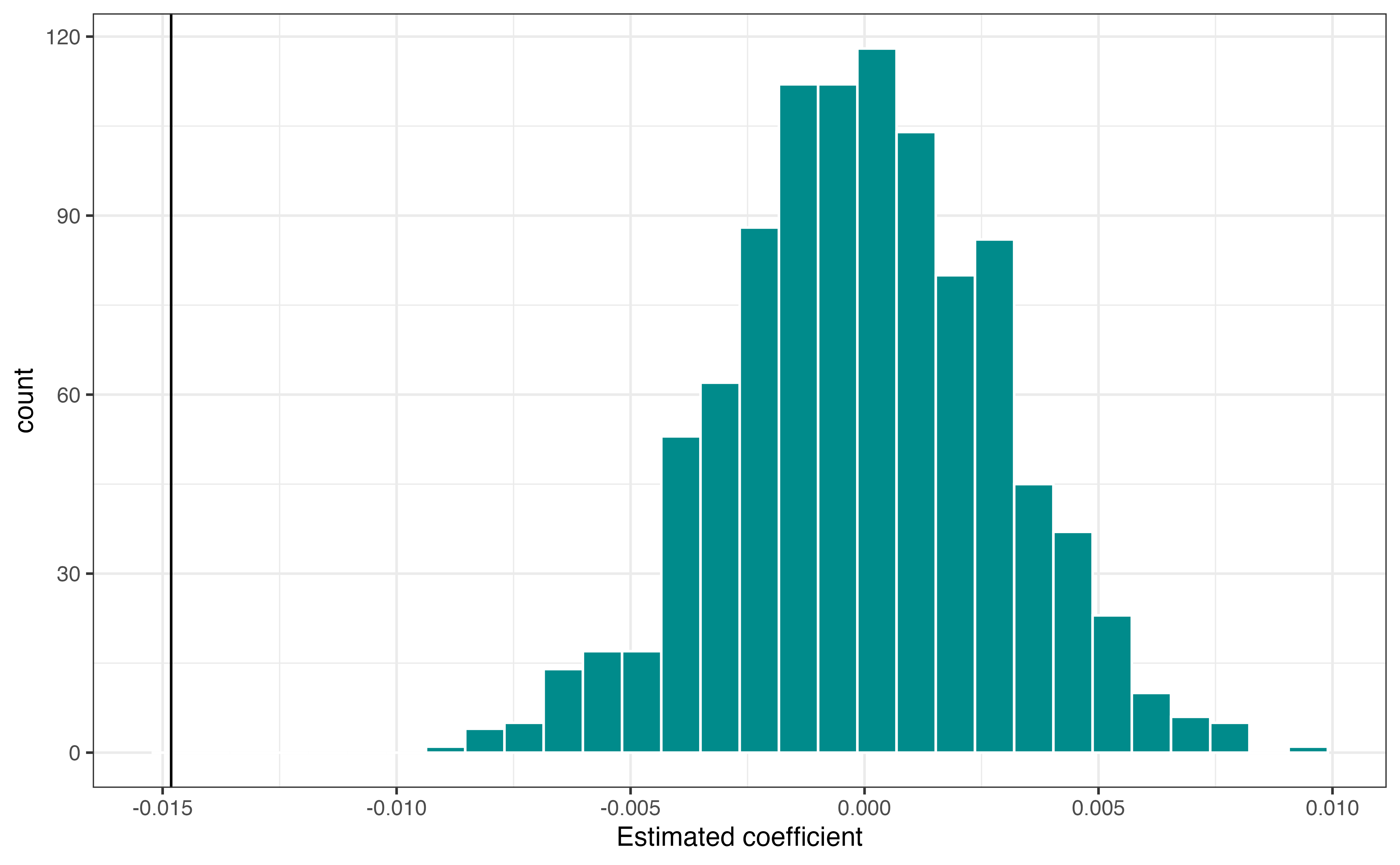
Figure 11.8 is the null distribution produced from the 1000 permutations.

Figure 11.8: Null distribution produced by permutation sampling. The solid line is the observed value of `age`.

Figure 11.8 shows that the estimated coefficient (solid vertical line) is far away from the center of the null distribution (the null hypothesized value 0), suggesting the evidence is not consistent with the null hypothesis. The p-value quantifies the strength of evidence against the null hypothesis. Based on the hypotheses in Equation 11.12, it is computed as the number of observations in the null distribution that have magnitude greater than $| β_{age} |$ .

The p-value in this example is $\approx$ 0. The p-value is very small, suggesting sufficient evidence against the null hypothesis. We reject the null hypothesis and conclude there is evidence of a relationship between age and comfort with driverless cars, after adjusting for opinions on technology.

Bootstrap confidence intervals

A confidence interval is a range of values in which a population parameter may reasonably take. This range of values is computed based on the sampling distribution of the estimated statistic. When conducting simulation-based inference, we use bootstrap sampling to construct this sampling distribution.

The process for constructing the sampling distribution using bootstrapping is the same for logistic regression as the process for linear regression in Section 5.4. Each bootstrap sample is constructed by sampling with replacement $n$ times, where $n$ is the number of observations in the sample data. The model is fit to each bootstrap sample, and the estimated coefficients make up the sampling distribution. The $C %$ confidence interval is computed as the bounds marking the middle $C %$ of the bootstrapped sampling distribution.

Figure 11.9 is the bootstrap sampling distribution for ${\hat{β}}_{age}$ for 1000 bootstrap samples.

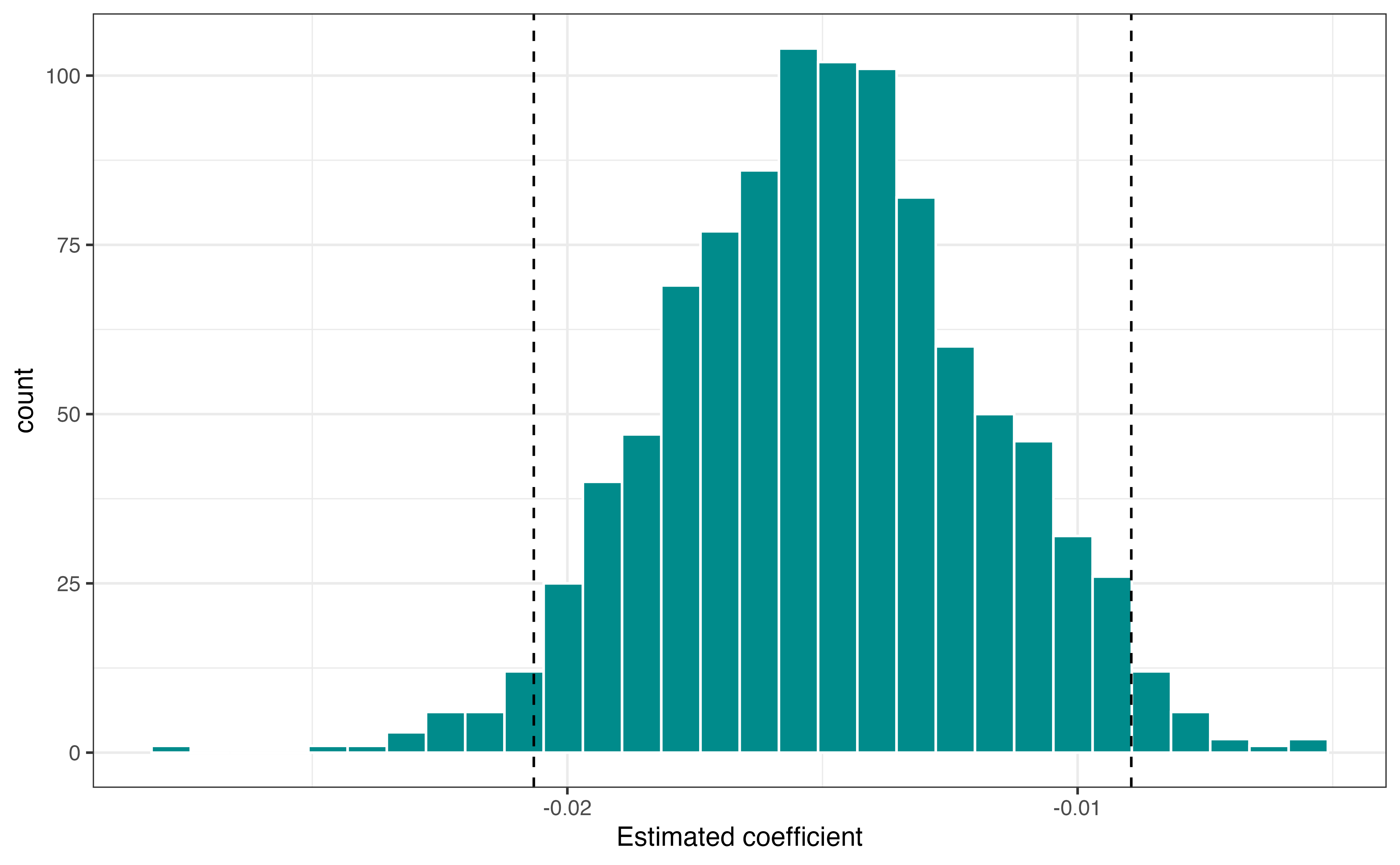
Figure 11.9: Bootstrap distribution for the coefficient of `age`. The vertical lines are the bounds for the 95% confidence interval.

The 95% bootstrap confidence is -0.021 to -0.009. These values are marked by vertical lines in Figure 11.9. As with the model output, these are in terms of the relationship between age and the log odds of being comfortable with driverless cars. Thus, the direct interpretation of the 95% confidence interval is as follows:

We are 95% confident that for each additional year in age, the log odds of being comfortable with driverless cars decrease between 0.009 to 0.021, holding opinions on technology constant.

The interpretation in terms of the odds is the following:

We are 95% confident that for each additional year in age, the odds of being comfortable with driverless cars multiply by a factor of 0.98 ( $e^{- 0.021}$ ) to 0.991 ( $e^{- 0.009}$ ), holding opinions on technology constant.

11.5.2 Theory-based inference

The general process for theory-based inference for a single coefficient in logistic regression is similar as linear regression. The primary difference is in the distribution of the estimated coefficient ${\hat{β}}_{j}$ .

When fitting a linear regression model, we have an formula for the estimated coefficients (see Section 4.4 and Section 7.3). Thus we have an exact formula for the distribution of a given coefficient ${\hat{β}}_{j}$ that applies for any sample size. Recall that we account for the sample size in how we define degrees of freedom of the $t$ distribution for the coefficients (see Section 8.4.1).

In logistic regression, the coefficients are estimated using maximum likelihood estimation (see Section 11.4), such that numerical optimization methods are used to find the combination of coefficients that maximize the likelihood function. There is no closed-form equation for the estimated coefficients as with linear regression. Because the estimated coefficients are approximated using optimization, the distribution of the coefficients are also approximated.

When the sample size is large , the distribution of the individual estimated coefficient ${\hat{β}}_{j}$ is $N (β_{j}, S E_{{\hat{β}}_{j}})$ , approximately normal with an expected value of $β_{j}$ , the true value of the coefficient and standard error $S E_{{\hat{β}}_{j}}$ . In practice, we will get the estimated standard error from the software output. Mathematical details about computing $S E_{{\hat{β}}_{j}}$ are described in Section B.3.

Hypothesis test

The steps for the hypotheses test are the same as those outlined in Section 8.4.2.

State the null and alternative hypotheses.
Calculate a test statistic.
Calculate a p-value.
Draw a conclusion.

The hypotheses for a single coefficient are the same as in Equation 11.12:

$H_{0} : β_{j} = 0 vs H_{a} : β_{j} \neq 0$

The test statistic, in Equation 11.13, is called the Wald test statistic (Wald 1943), because it is based on the approximation of the mean and standard error as $n$ is large.

$\begin{matrix} (11.13) & z = \frac{{\hat{β}}_{j} - 0}{S E_{{\hat{β}}_{j}}} \end{matrix}$

The test statistic, denoted by $z$ , is the number of standard errors the estimated coefficient ${\hat{β}}_{j}$ is from 0, the hypothesized mean of the distribution. It follows a standard normal distribution, $N (0, 1)$ , because it is based on asymptotic results (compared to the $t$ test statistic in linear regression which applies even for small $n$ ). Because the alternative hypothesis is two-sided, the p-value is computed as $P (| Z | \geq | z |)$ , where $Z \sim N (0, 1)$ . The p-value is interpreted as before, with small p-values providing stronger evidence against the null hypothesis.

Let’s take a look at the hypothesis test for the coefficient of age using the theory-based methods. The components for the theory-based hypothesis test are produced in the model output. The output of the model including tech_easy and age is reproduced in Table 11.7 along with the 95% confidence intervals for the model coefficients.

Table 11.7: Model output for aidrive_comfort versus tech_easy and age with 95% confidence intervals for coefficients

term	estimate	std.error	statistic	p.value	conf.low	conf.high
(Intercept)	0.420	0.208	2.020	0.043	0.012	0.828
tech_easyCan’t choose	-0.118	0.402	-0.294	0.769	-0.928	0.661
tech_easyAgree	0.678	0.151	4.487	0.000	0.383	0.976
tech_easyDisagree	-0.499	0.295	-1.690	0.091	-1.094	0.068
age	-0.015	0.003	-4.902	0.000	-0.021	-0.009

The hypotheses are the same as with simulation-based inference

$H_{0} : β_{age} = 0 vs β_{age} \neq 0$

The null hypothesis is that there is no relationship between age and comfort with driverless cars after accounting for opinions about technology. The alternative hypothesis is that there is a relationship.

The test statistic⁸ is computed as

$z = \frac{- 0.015 - 0}{0.003} \approx - 5$

The p-value is computed as $P (| Z | \geq | - 4.902 |) \approx$ 4.83^{-6}. This value is so small it rounds to 0 when displaying the results to 3 digits. This is consistent with the p-value we observed from the permutation test in Section 11.5.1. Because the p-value is small, we reject the null hypothesis and conclude there is evidence of a relationship between age and comfort with driverless cars after adjusting for opinions about technology.

We can use a decision-making threshold $α$ when using the p-value to draw conclusions from a hypothesis test. The potential for Type I and Type II errors is the same for logistic regression as in linear regression. See Section 5.6.4 for more on choosing $α$ and potential errors.

Confidence interval

The equation to compute the confidence interval for coefficients in logistic regression is very similar to the formula in linear regression from Section 5.8. The difference is the critical value $z^{*}$ is computed from the $N (0, 1)$ distribution

$\begin{matrix} (11.14) & {\hat{β}}_{j} \pm z^{*} \times S E_{{\hat{β}}_{j}} \end{matrix}$

In practice, the confidence interval is produced in the model output. Let’s show how the 95% confidence interval for age is computed in Table 11.7.

The values for ${\hat{β}}_{j}$ and $S E_{{\hat{β}}_{j}}$ can be read directly from table, as before. The critical value $z^{*}$ is the point on the $N (0, 1)$ distribution such that the middle 95% (or $C %$ in general) of the distribution is between $- z^{*}$ and $z^{*}$ . We can use statistical software to get this value as shown in Section 11.7. The $z^{*}$ for the 95% confidence interval is 1.96.

The 95% confidence interval for the coefficient of age is

$\begin{aligned} - 0.015 \pm 1.96 \times 0.003 \\ \Rightarrow & - 0.015 \pm 0.00588 \\ \Rightarrow & [- 0.021, - 0.009] \end{aligned}$

Interpret this interval in the context of the data in terms of the odds of being comfortable with driverless cars.
How does this interval compare to the bootstrap confidence interval computed in Section 11.5.1? ⁹

Connection between hypothesis test and confidence intervals

The same connection between two-sided hypothesis tests and confidence intervals applies in the context of logistic regression as we saw in linear regression in Section 5.7 . A two-sided hypothesis test with decision-making threshold of $α$ directly corresponds to the $(1 - α) \times 100 %$ confidence interval. For example, a hypothesis test with decision-making threshold of $α = 0.05$ directly corresponds to the 95% ( $(1 - 0.05) \times 100$ ) confidence interval.

This means we can use a confidence interval to evaluate a claim about a coefficient and get a range of values the population coefficient may take. The following are the relationship between the confidence interval and hypothesis test:

Confidence interval for $β_{j}$ : If 0 is in the interval, fail to reject the null hypothesis. If 0 is not in the interval, reject the null hypothesis.
Confidence interval for $e^{β_{j}}$ : If 1 is in the interval, fail to reject the null hypothesis. If 1 is not in the interval, reject the null hypothesis.

Use the output in Table 11.7.

Show how the test statistic is computed for tech_easyDisagree. Interpret this value in the context of the data.
Do the data provide evidence that the odds are different among those who disagree technology makes life easier compared to those who are neutral (the baseline), after adjusting for age? Use $α = 0.05$ Explain.
Show how the 95% confidence interval for tech_easyDisagree is computed. Is it consistent with your conclusion in the previous question?¹⁰

11.6 Model conditions

We fit logistic regression model under a set of assumptions. These are similar to the assumptions for linear regression in Section 5.3, but there is no assumption related to normality or equal variance.

There is a linear relationship between the predictors and logit of the response variable
The observations are independent of one another

Similar to linear regression, we check model conditions to evaluate whether these assumptions hold for the data.

11.6.1 Linearity

The linearity assumption for logistic regression states that there is a linear relationship between the predictors and the logit of the response variable. We check this assumption by looking at plots of the quantitative predictors versus the empirical logit of the response. The empirical logit is the log-odds of a binary variable (“logit”) calculated from the data (“empirical”). For example, Equation 11.15 is the empirical logit for the comfort with driverless cars in the sample data set.

$\begin{matrix} (11.15) & empirical logit = \log (\frac{π}{1 - π}) = \log (\frac{0.545}{1 - 0.545}) = 0.180 \end{matrix}$

We can also look at the empirical logit by subgroup of a categorical variable. For example, Table 11.8 shows the empirical logit by opinion on whether technology makes life easier.

Table 11.8: Probability and empirical logit of aidrive_comfort by tech_easy

tech_easy	n	Probability	Empirical Logit
Neutral	217	0.415	-0.344
Can’t choose	30	0.400	-0.405
Agree	1201	0.588	0.355
Disagree	73	0.288	-0.907

Computing the empirical logit across values of a quantitative predictor is similar as the process for categorical predictors. We divide the values of the quantitative predictor into bins and compute the empirical logit of the response for the observations within each bin. There are multiple ways to divide the quantitative predictor into bins. Some software creates the bins, such that there are an equal number of observations in each bin. Another option is to create bins by dividing by some incremental amount (e.g., dividing age into 5 or 10 year increments). Dividing the variable by the same incremental amount can be more easily interpreted; however, there may be large variation in the number of observations in each bin that needs to be taken into account when comparing the empirical logit across bins. The former method may be less interpretable, but we know the empirical logit is computed using the same observations for each bin.

Table 11.9 shows the number of observations $n$ , probability, and empirical logit across bins of age using the two approaches for dividing age into bins. In Table (a) of Table 11.9, the bins have been created such that the observations are more evenly distributed across bins. Often, the number of observations will be equal or differ by a small amount. In this case, because age is a discrete variable, there are many observations with the exact same value of age. For example, there are 38 observations with the age of 39 years old. Because all observations with the same age are in the same bin, the number of observations in bins that include ages that occur frequently is higher than less common ages in the data, such as those over 70 years old. Note, however, that the number of observations in each bin are still more even than when the bins are created using equal age increments.

Table 11.9: Probability and empirical logit of aidrive_comfort by age

(a) Evenly distribute observations

age_bins	n	Probability	Empirical Logit
[18,27)	158	0.677	0.741
[27,34)	154	0.636	0.560
[34,40)	178	0.607	0.434
[40,45)	141	0.582	0.329
[45,50)	134	0.575	0.301
[50,57)	157	0.490	-0.038
[57,63)	153	0.438	-0.250
[63,69)	163	0.466	-0.135
[69,75)	143	0.462	-0.154
[75,89]	140	0.507	0.029

(b) Equal age increments

age_bins	n	Probability	Empirical Logit
(18,25]	132	0.667	0.693
(25,32]	151	0.642	0.586
(32,39]	207	0.618	0.483
(39,46]	193	0.549	0.198
(46,54]	159	0.572	0.291
(54,61]	188	0.463	-0.149
(61,68]	181	0.448	-0.211
(68,75]	170	0.471	-0.118
(75,82]	90	0.567	0.268
(82,89]	50	0.400	-0.405

Now that we can compute the empirical logit, let’s use it to check the linearity assumption. As with linear regression, we only check linearity for quantitative predictors. To check linearity, we will make a plot of the empirical logit of the response versus the bins of the quantitative predictor. We use the mean value within each bin of the predictor to represent the bin on the graph.

Figure 11.10 shows a plot of the empirical logit of being comfortable with driverless cars versus the mean value of age in each bin. We use the bins from Table (a) in Table 11.9, so that we know there is a similar number of observations represented by each point on the graph.

Figure 11.10: Empirical logit of `aidrive_comfort` versus `age`

When examining the plot of empirical logit versus the binned quantitative predictor, we are asking whether a line would reasonably describe the relationship between the predictor and empirical logit. The condition is satisfied if the trend generally looks linear overall. As with checking the linearity condition for linear regression, we are looking for obvious violations, not exact adherence to linearity.

From Figure 11.10, it appears there is a potential quadratic relationship between age and comfort with driverless cars, and thus the linearity condition is not satisfied. The empirical logit is lowest for respondents around 60 years old, then it appears to increase again. This prompts us to consider a quadratic term for the model.

Table 11.10: Logistic regression model including quadratic term for age.

term	estimate	std.error	statistic	p.value	conf.low	conf.high
(Intercept)	1.2106	0.4545	2.664	0.0077	0.3246	2.1077
tech_easyCan’t choose	-0.1600	0.4040	-0.396	0.6922	-0.9745	0.6227
tech_easyAgree	0.6832	0.1512	4.519	0.0000	0.3884	0.9816
tech_easyDisagree	-0.5118	0.2956	-1.731	0.0834	-1.1070	0.0562
age	-0.0498	0.0181	-2.755	0.0059	-0.0854	-0.0145
I(age^2)	0.0003	0.0002	1.967	0.0492	0.0000	0.0007

Table 11.10 is the output of the model that includes the quadratic term for age. The p-value for the quadratic term is around 0.05, so based on this alone, it is unclear whether or not to keep the squared term in the model. Thus, let’s look at the confidence interval and some model comparison statistics introduced in Section 10.2 to have more information to take into account regarding the quadratic term.

The 95% confidence interval for the coefficient of ${age}^{2}$ is 1.955^{-6} to 6.802^{-4}. This shows the quadratic term has a very small adjustment on the relationship between age and comfort with driverless cars. Even if the quadratic term is statistically significant, it may not be practically significant.

Table 11.11: AIC and BIC for models with and without quadratic term for age

Model	AIC	BIC
Age	2036	2062
Age + Age^2	2034	2066

In Table 11.11, we look at the AIC and BIC for the model with and without the quadratic term for age. The model that includes ${age}^{2}$ has a lower AIC but a higher BIC. The difference in the AIC values is small, indicating that that one model is not preferenced over the other in terms of model fit. The same is true when comparing the values of BIC. Therefore, with a mind towards choosing the most parsimonious (simplest) model without hindering model performance, we choose to remove the quadratic term and move forward including only the main effect for age.

11.6.2 Independence

The independence assumption for logistic regression is similar to the assumption for linear regression, that there are no dependencies between observations. As with linear regression, this assumption is important, because we conduct inference assuming we have $n$ pieces of independent information produced by the $n$ observations. If observations there is dependency between observations, then we are effectively working with less than $n$ pieces of independent information, as knowing something about one observation tells a lot about all the others that are correlated with it.

We typically evaluate independence based on a description of the observations and the data collection process. If there are potential dependency issues based on the order in which the data were collected, spatial correlation, or other sub group dependencies, we can use visualizations to plot the odds or empirical logit of the response by time, space, or subgroup, respectively. We can also add predictors in the model to account for those potential dependencies.

For this analysis on comfort with driverless cars, the independence condition is satisfied. Based on the description of the sample and data collection process in Section 11.1, we can reasonably conclude there are no dependencies between respondents.

We conduct logistic regression assuming the data are a representative sample from the population of interest. Ideally, it would be a random sample, but that is not always feasible in practice. Therefore, even if the sample is not completely random, it should be representative of the population.

If there are biases in the sample (e.g., a particular subgroup is over or under represented in the data), they will influence the interpretations, conclusions, and predictions from the model. Therefore, we can narrow the scope of the population for the analysis, or clearly disclose these biases when presenting the results.

This issue often occurs in survey data, like the data we’re analyzing in this chapter. Data scientists analyzing survey data will often include weights in their analysis so that the sample looks more representative of the population in the analysis calculations even if the original data has some bias.

11.7 Logistic regression in R

11.7.1 Fitting a logistic model

The logistic regression model is fit using glm() in the stats package in base R. This function is used to fit a variety of models that are part of the wider class of models called generalized linear models, so we must also specify which generalized linear model is being fit when using this function. The argument family = binomial is specifies that the model fit is a logistic regression model.

comfort_tech_age_fit <- glm(aidrive_comfort ~ tech_easy + age,
                          data = gss24_ai, 
                          family = binomial)

We input the observed categorical response variable and R does all computations behind the scenes to produce the model in terms of the logit. The response variable must be coded as a character (<chr>) or factor (<fct>) type.

The tidy function produces the model output in a tidy form and kable() can be used to neatly format the results to a specific number of digits. The argument conf.int = TRUE shows the confidence interval, and conf.level = is used to set the confidence level.

tidy(comfort_tech_age_fit, conf.int = TRUE ,conf.level = 0.95) |>
  kable(digits = 3)

term	estimate	std.error	statistic	p.value	conf.low	conf.high
(Intercept)	0.420	0.208	2.020	0.043	0.012	0.828
tech_easyCan’t choose	-0.118	0.402	-0.294	0.769	-0.928	0.661
tech_easyAgree	0.678	0.151	4.487	0.000	0.383	0.976
tech_easyDisagree	-0.499	0.295	-1.690	0.091	-1.094	0.068
age	-0.015	0.003	-4.902	0.000	-0.021	-0.009

By default, the tidy function will show the model output for the response in terms of the logit. The argument exponentiate = TRUE will produce the output for the model in terms of the odds with the exponentiated coefficients. The argument, exponentiate is set to FALSE by default.

tidy(comfort_tech_age_fit, conf.int = TRUE ,conf.level = 0.95, 
     exponentiate = TRUE) |>
  kable(digits = 3)

term	estimate	std.error	statistic	p.value	conf.low	conf.high
(Intercept)	1.522	0.208	2.020	0.043	1.012	2.289
tech_easyCan’t choose	0.889	0.402	-0.294	0.769	0.395	1.936
tech_easyAgree	1.969	0.151	4.487	0.000	1.467	2.653
tech_easyDisagree	0.607	0.295	-1.690	0.091	0.335	1.071
age	0.985	0.003	-4.902	0.000	0.979	0.991

11.7.2 Simulation-based inference

The code for simulation-based inference is the same for logistic regression as the code for linear regression introduced in Section 4.8. Behind the scenes, the functions in the infer R package use the response variable to determine whether to fit a linear or logistic regression model.

Below is the code for the bootstrap confidence intervals and permutation test conducted in Section 11.5.1. We refer the reader to Section 8.7.1 for more a more detailed explanation about the code.

Permutation test

# set seed
set.seed(12345)

# construct null distribution using permutation sampling
null_dist <- gss24_ai |> 
  specify(aidrive_comfort ~ tech_easy + age) |>
  hypothesize(null = "independence") |>
  generate(reps = 1000, type = "permute", variables = age) |>
  fit()

# compute observed coefficient
obs_fit <- gss24_ai |> 
  specify(aidrive_comfort ~ tech_easy + age) |> 
  fit()

# compute p-value
pval <- get_p_value(null_dist, obs_stat = obs_fit, direction = "two-sided")

Bootstrap confidence interval

# set seed
set.seed(12345)

# construct bootstrap distribution 
boot_dist <- gss24_ai |>
  specify(aidrive_comfort ~ tech_easy + age) |>
  generate(reps = 1000, type = "bootstrap") |>
  fit()

# compute confidence interval
ci <- get_confidence_interval(
    boot_dist, 
    level = 0.95, 
    point_estimate = obs_fit
  )

11.7.3 Empirical logit plots

The code to compute the empirical logit primarily utilizes data wrangling functions in the dplyr R package (Wickham et al. 2023a).

Empirical logit for groups of a categorical variable

The code below produces the empirical logit for being comfortable with driverless cars for each level of tech_easy, opinion on whether technology makes life easier.

1gss24_ai |>
2  group_by(tech_easy) |>
3  count(aidrive_comfort) |>
4  mutate(probability = n / sum(n),
         empirical_logit = log(probability/(1 - probability)))

1: Use the gss24_ai data frame.
2: Compute all subsequent calculations separately for each level of tech_easy.
3: Count the number of observations such that aidrive_comfort == 0, and the number of observations such that aidrive_comfort == 1.
4: Compute the probability that aidrive_comfort == 0 and aidrive_comfort == 1 .

# A tibble: 8 × 5
# Groups:   tech_easy [4]
  tech_easy    aidrive_comfort     n probability empirical_logit
  <fct>        <fct>           <int>       <dbl>           <dbl>
1 Neutral      0                 127       0.585           0.344
2 Neutral      1                  90       0.415          -0.344
3 Can't choose 0                  18       0.6             0.405
4 Can't choose 1                  12       0.4            -0.405
5 Agree        0                 495       0.412          -0.355
6 Agree        1                 706       0.588           0.355
# ℹ 2 more rows

The code to compute the empirical logit based on a quantitative predictor is the similar, with the additional step of splitting the quantitative predictor into bins. There are many ways to do this in R; here we will show the functions used for the tables in Section 11.6.

The first is using the cut() function that is part of base R. This function transforms numeric variable types into factor variable types by dividing them into bins. The argument breaks = is used to either specify the number of bins or explicitly define the bins. If the number of bins is specified, cut() will divide the observations into bins of equal length, as shown in the code below.

Once the bins are defined, the remainder of the code is the same as before, where the probability and empirical logit are computed for each bin. Here is the code to compute the empirical logit of comfort with driverless cars by age, where age is divided into 10 bins. Here, the cut() function divided the age into bins of length 7.

Note that the option dig.lab = 0 in the cut() function means to display the bin thresholds as integers, i.e., with 0 digits. This only changes how the lower and upper bounds are displayed; it does not change any computations.

gss24_ai |> 
  mutate(age_bins = cut(age, breaks = 10, dig.lab = 0)) |>
  group_by(age_bins) |>
  count(aidrive_comfort) |>
  mutate(probability = n / sum(n)) |>
  mutate(empirical_logit = log(probability/(1 - probability)))

# A tibble: 20 × 5
# Groups:   age_bins [10]
  age_bins aidrive_comfort     n probability empirical_logit
  <fct>    <fct>           <int>       <dbl>           <dbl>
1 (18,25]  0                  44       0.333          -0.693
2 (18,25]  1                  88       0.667           0.693
3 (25,32]  0                  54       0.358          -0.586
4 (25,32]  1                  97       0.642           0.586
5 (32,39]  0                  79       0.382          -0.483
6 (32,39]  1                 128       0.618           0.483
# ℹ 14 more rows

Another option for splitting the quantitative variable into bins is to do, such that each bin has an approximately equal number of observations. To do so, we can use the cut2() function from them Hmisc R package (Harrell Jr 2025). The number of bins is specified in the g = argument, and the function will divide the observations into the number of specified bins, such that each bin has an approximately equal number of observations.

gss24_ai |> 
  mutate(age_bins = cut2(age, g = 10)) |>
  group_by(age_bins) |>
  count(aidrive_comfort) |>
  mutate(probability = n / sum(n)) |>
  mutate(empirical_logit = log(probability/(1 - probability))) |>
  filter(aidrive_comfort == 1)

# A tibble: 10 × 5
# Groups:   age_bins [10]
  age_bins aidrive_comfort     n probability empirical_logit
  <fct>    <fct>           <int>       <dbl>           <dbl>
1 [18,27)  1                 107       0.677          0.741 
2 [27,34)  1                  98       0.636          0.560 
3 [34,40)  1                 108       0.607          0.434 
4 [40,45)  1                  82       0.582          0.329 
5 [45,50)  1                  77       0.575          0.301 
6 [50,57)  1                  77       0.490         -0.0382
# ℹ 4 more rows

We see the bins are more evenly distributed than using the previous method, but there is not an equal number in each bin. This is because the data set is imbalanced, as there are many more respondents in the data who are 18 - 27 years old versus 75 years and older. We can try different values for g = (minimum of 5), if we wish to make the bins more evenly distributed.

The plot of the empirical logit versus a quantitative predictor has the mean value within each bin on the $x$ -axis and the empirical logit for the bin on the $y$ -axis. In the code below, we use the summarise() function in the dplyr R package (Wickham et al. 2023b) to compute the mean age within each bin. We then join the mean ages to the empirical logit data computed above (saved as the object emplogit_age), and use the combined data to create the scatterplot.

# compute mean age for each bin
mean_age  <- gss24_ai |> 
  mutate(age_bins = cut(age, breaks = 10)) |> 
  group_by(age_bins) |>
  summarise(mean_age = mean(age))

# join the mean ages and create scatterplot
emplogit_age |> 
  left_join(mean_age, by = "age_bins") |>
  ggplot(aes(x = mean_age, y = empirical_logit)) +
  geom_point() +
  labs(x = "Mean age", 
       y = "Empirical logit of (aidrive_comfort = 1)") +
  theme_bw()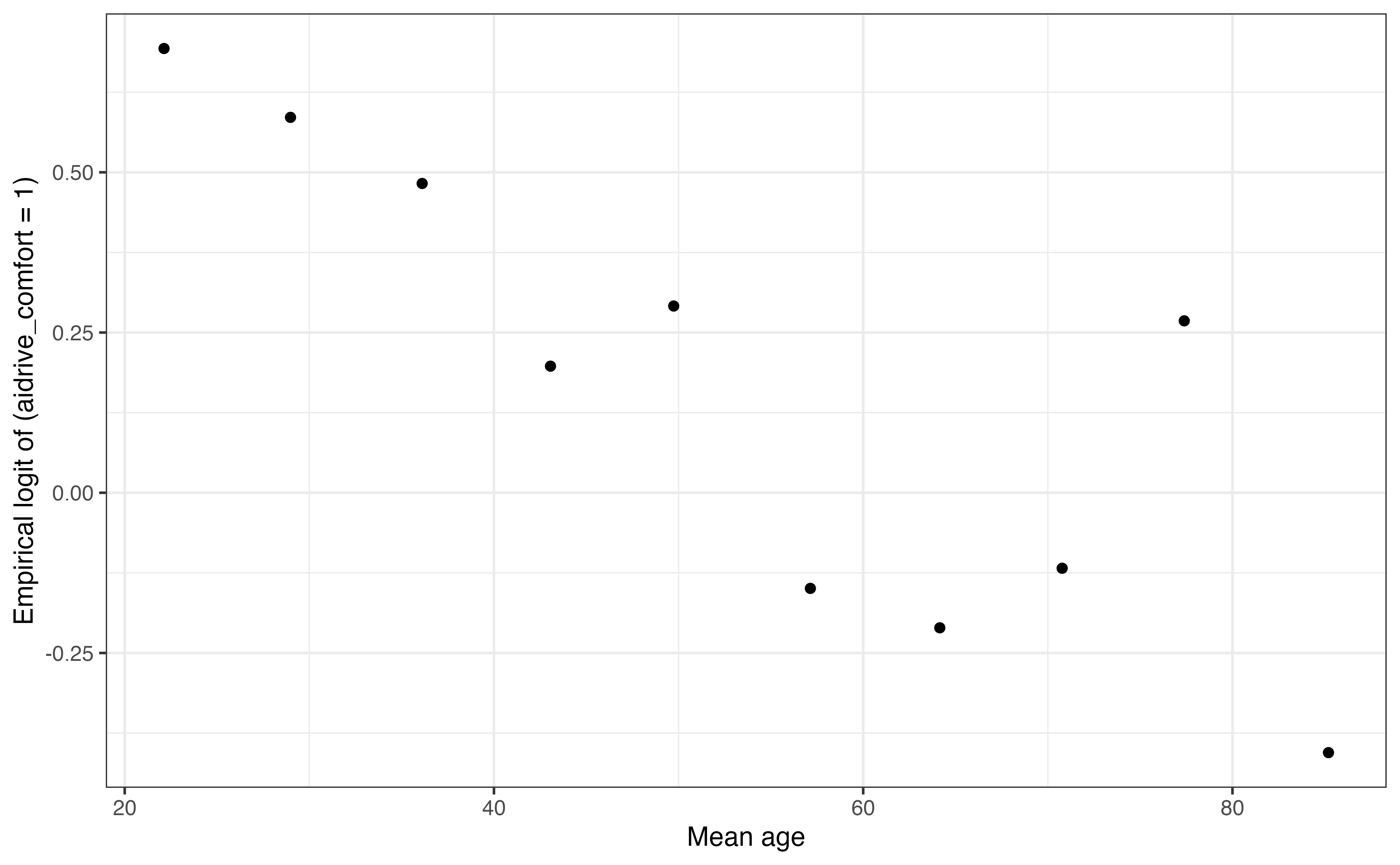

The Stat2Data R package (Cannon et al. 2019) has built-in functions for making empirical logit plot utilizing the base R plotting functions (instead of ggplot2).

The emplogitplot1() function is used to create the empirical logit plot for the response versus a quantitative predictor variable. The argument ngroups = specifies the number of bins. The bins can be explicitly defined using the breaks= argument instead of ngroups.

The code for the empirical logit plot versus age using 10 bins is below.

emplogitplot1(aidrive_comfort ~ age, data = gss24_ai, ngroups = 10)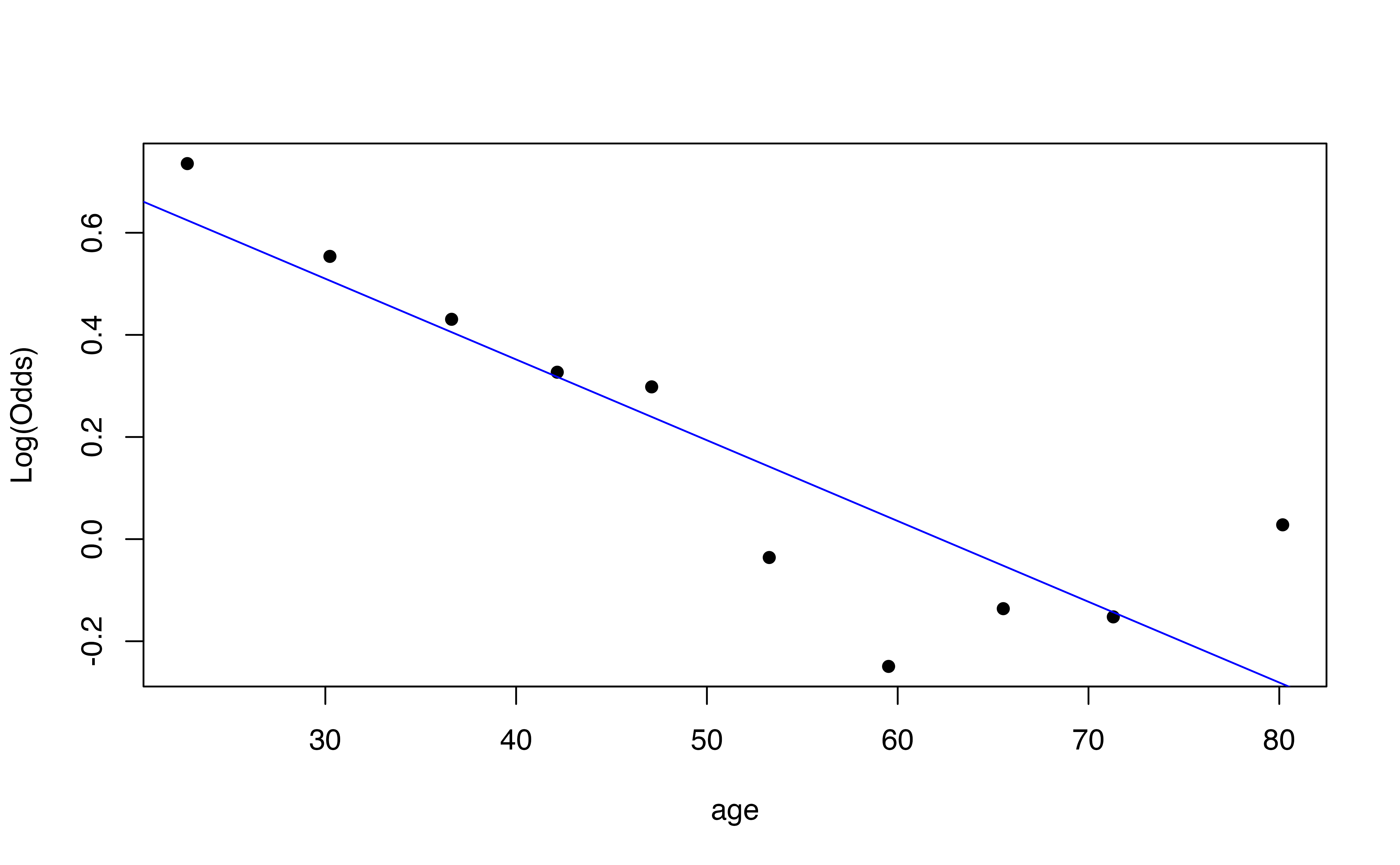

We can include the argument out = TRUE save the underlying data used to make the plot. Additionally, the argument showplot = FALSE will suppress the plot, if we are only interested in the underlying data.

emplogit_age_data <- emplogitplot1(aidrive_comfort ~ age, data = gss24_ai, 
                                   ngroups = 10, out = TRUE, showplot = FALSE)

emplogit_age_data

   Group Cases XMin XMax XMean NumYes  Prop AdjProp  Logit
1      1   158   18   26  22.8    107 0.677   0.676  0.735
2      2   154   27   33  30.2     98 0.636   0.635  0.554
3      3   178   34   39  36.6    108 0.607   0.606  0.431
4      4   141   40   44  42.2     82 0.582   0.581  0.327
5      5   134   45   49  47.1     77 0.575   0.574  0.298
6      6   157   50   56  53.3     77 0.490   0.491 -0.036
7      7   153   57   62  59.5     67 0.438   0.438 -0.249
8      8   163   63   68  65.5     76 0.466   0.466 -0.136
9      9   143   69   74  71.3     66 0.462   0.462 -0.152
10    10   140   75   89  80.2     71 0.507   0.507  0.028

As we see from the output of underlying data, emplogitplot1() divides the quantitative variable into bins, such that the observations are approximately evenly distributed across bins. The result is very similar to the result from creating bins using cut2(). The underlying data in emplogit_age_data can be used to make the graph using the ggplot2 functions, as shown below.

ggplot(emplogit_age_data, aes(x = XMean, y = Logit )) + 
  geom_point() + 
    labs(x = "Mean age", 
       y = "Empirical logit of (aidrive_comfort = 1)") +
  theme_bw()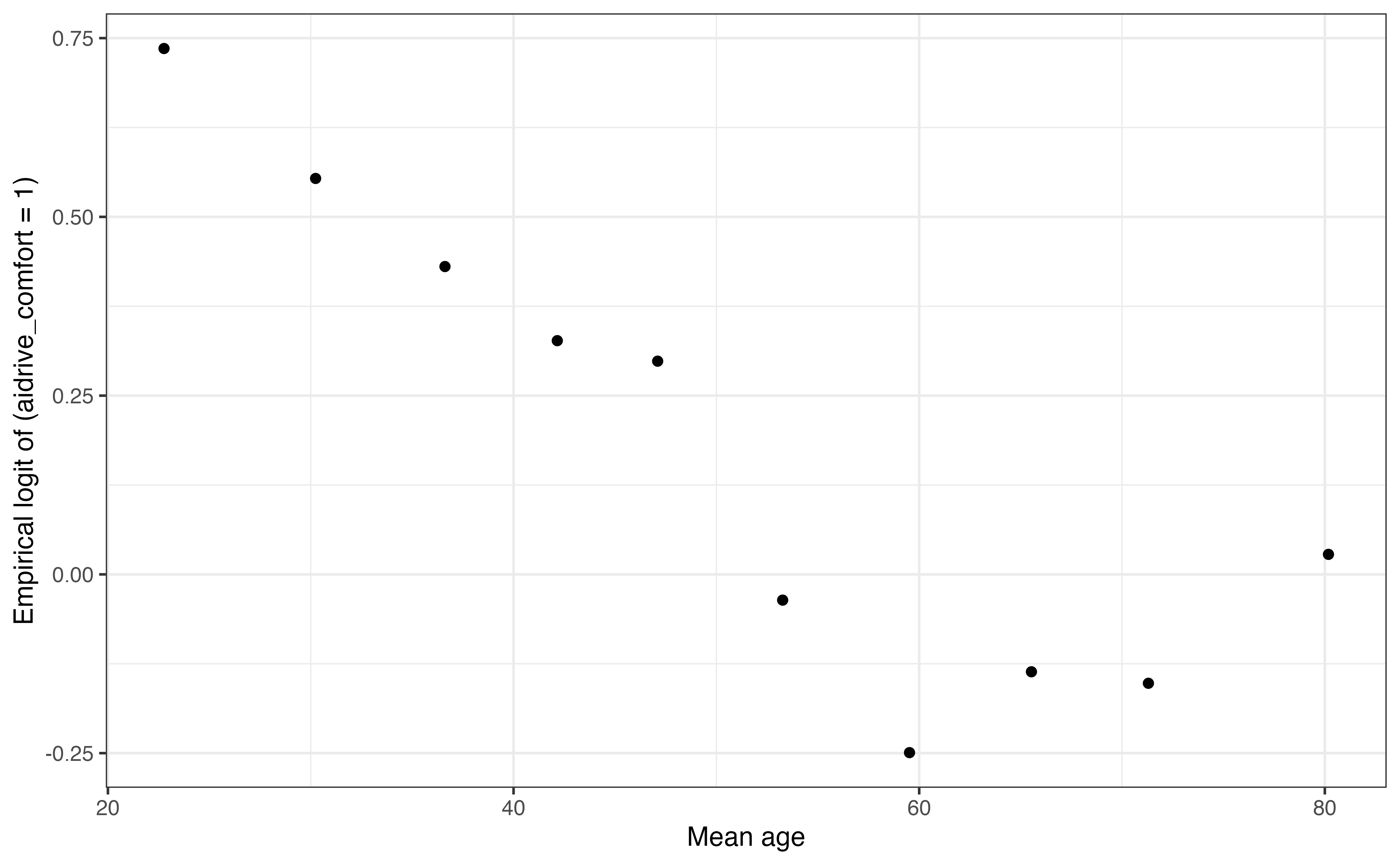

11.8 Summary

In this chapter we introduced logistic regression for data with a binary categorical response variable. We used probabilities and odds to describe the distribution of the response variable, and we used odds ratios to understand the relationship between the response and predictor variables. We introduced the form of the logistic regression model and interpreted the model coefficients in terms of the logit and odds. We used simulation-based and theory-based methods to draw conclusions about individual coefficients, and used model conditions to evaluate whether the assumptions for logistic regression hold in the data. We concluded by showing these elements of logistic regression analysis in R.

In Chapter 12, we will continue with logistic regression models and show how these models are used for prediction and classification. We will also present statistics to evaluate model fit and conduct model selection.

There does appear to be some relationship. A higher proportion of those who agree technology makes life easier have comfort with driverless cars.↩︎
$P r (Y = 1) = 829 / (692 + 829) = 0.545$

$odds (Y = 1) = 0.545 / (1 - 0.545) \approx 1.2$

Note results differ slightly due to rounding.↩︎
$P r (Y = 1 | tech_easy = Agree) = 706 / (495 + 706) = 0.588$ and $odds (Y = 1 | tech_easy = Agree) = 0.588 / (1 - 0.588) = 706 / 495 = 1.43$ ↩︎
The odds ratio is $\frac{706 / 495}{21 / 52} = 3.53$ . This means that the odds a respondent who agrees technology makes life easier is comfortable with driverless cars are 3.53 times the odds a respondent who is disagrees that technology is making life easier is comfortable with driverless cars.↩︎
The baseline level is Neutral . It is the only level that is not in the model output.↩︎
The log odds a respondent who disagrees technology makes life easier is comfortable with driverless cars are expected to be 0.499 less than the log odds of a respondent who is neutral about whether technology makes life easier, holding age constant.

The odds a respondent who disagrees technology makes life easier is comfortable with driverless cars are expected to be 0.607 ( $e^{- 0.499}$ ) times the odds of a respondent who is neutral about whether technology makes life easier, holding age constant.

Alternatively, we could write this in terms of an odds ratio greater than 1: The odds a respondent is neutral about whether technology makes life easier is comfortable with driverless cars are expected to be 1.647 ( $1 / e^{- 0.499}$ ) times the odds of a respondent who disagrees that technology makes life easier, holding age constant.↩︎
When age increases by 5, the log odds are expected to decrease by 0.075 ( $- 0.015 \times 5$ ) . The odds are expected to multiply by 0.928 ( $e^{- 0.015 \times 5}$ ).↩︎
Note the difference the result here and the model output is because the model output is computed using exact values of ${\hat{β}}_{j}$ and $S E_{{\hat{β}}_{j}}$ .↩︎
We are 95% confident that for each additional year in age, the odds of being comfortable with driverless cars are expected to multiply by 0.979 ( $e^{- 0.021}$ ) to 0.991 ( $e^{- 0.009}$ ), holding opinions about technology constant. This interval is equal to the interval obtained using bootstrapping.↩︎
- The test statistic is $\frac{- 0.499 - 0}{0.295} \approx - 1.69$ . The estimated coefficient of -0.499 is 1.69 standard errors below the hypothesized mean of 0. The p-value 0.091 > 0.05, so the data do not provide sufficient evidence the odds are different for those who disagree that technology makes life easier versus those who are neutral, after adjusting for age. The 95% confidence interval is computed as $- 0.499 \pm 1.96 \times 0.295$ . It is consistent with the conclusion, because 0 is in the interval.
↩︎