7  Multiple linear regression

Learning goals

• Explain how multiple predictor variables can be used to explain variability and predict a quantitative response variable
• Interpret model coefficients in the context of the data
• Compute predicted values from the multiple linear regression model
• Use different types of predictors in the regression model
• Conduct multiple linear regression analysis using R

7.1 Introduction: Lemurs

About 95% of lemur species are at risk of extinction, so it is important for researchers to study and better understand lemurs to more effectively save these species (Community 2024). The Duke Lemur Center currently has over 250 lemurs from 12 species. It has the most diverse population of lemurs outside of Madagascar, the native home for lemurs (Duke Lemur Center n.d.). In this chapter, we will use various characteristics to understand the variability in the weight of lemurs who are 24 months old or younger. We refer to this group of lemurs as “young lemurs” throughout the analysis. The data contains the weight and other features of young lemurs from three taxon (ERUF, PCOQ, and VRUB) who lived at the Duke Lemur Center at the time the data were collected. The data were originally from Zehr et al. (n.d.) and were featured as part of the TidyTuesday weekly data visualization challenge in August 2021 (Community 2024).

Eulemur rufus (ERUF)

Propithecus coquereli (PCOQ)

Varecia rubra (VRUB)

Figure 7.1: Types of lemurs represented in the data set. Images from Duke Lemur Center (n.d.).

The data are in lemurs-sample-young.csv. This analysis in this chapter focuses on the following variables:

• weight: Weight of the lemur (in grams)
• taxon : Code made as a combination of the lemur’s genus and species. Note that the genus is a broader categorization that includes lemurs from multiple species. This analysis focuses on the following taxon:

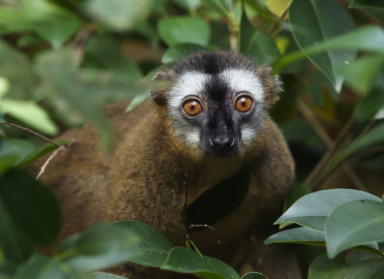
  • ERUF: Eulemur rufus, commonly known as Red-fronted brown lemur

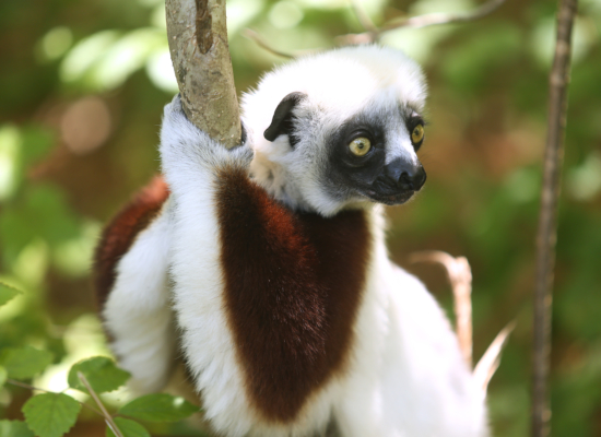
  • PCOQ: Propithecus coquereli, commonly known as Coquerel’s sifaka

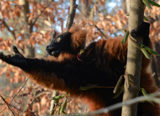
  • VRUB: Varecia rubra, commonly known as Red ruffed lemur

• sex : Sex of lemur (M: Male, F: Female)
• age: Age of lemur when weight was recorded (in months)
• litter_size: Total number of infants in the litter the lemur was born into (this includes the observed lemur)

The goal of the analysis is to use age, taxon, sex, and litter size to predict and explain variability in the weights of young lemurs.

7.1.1 Exploratory data analysis

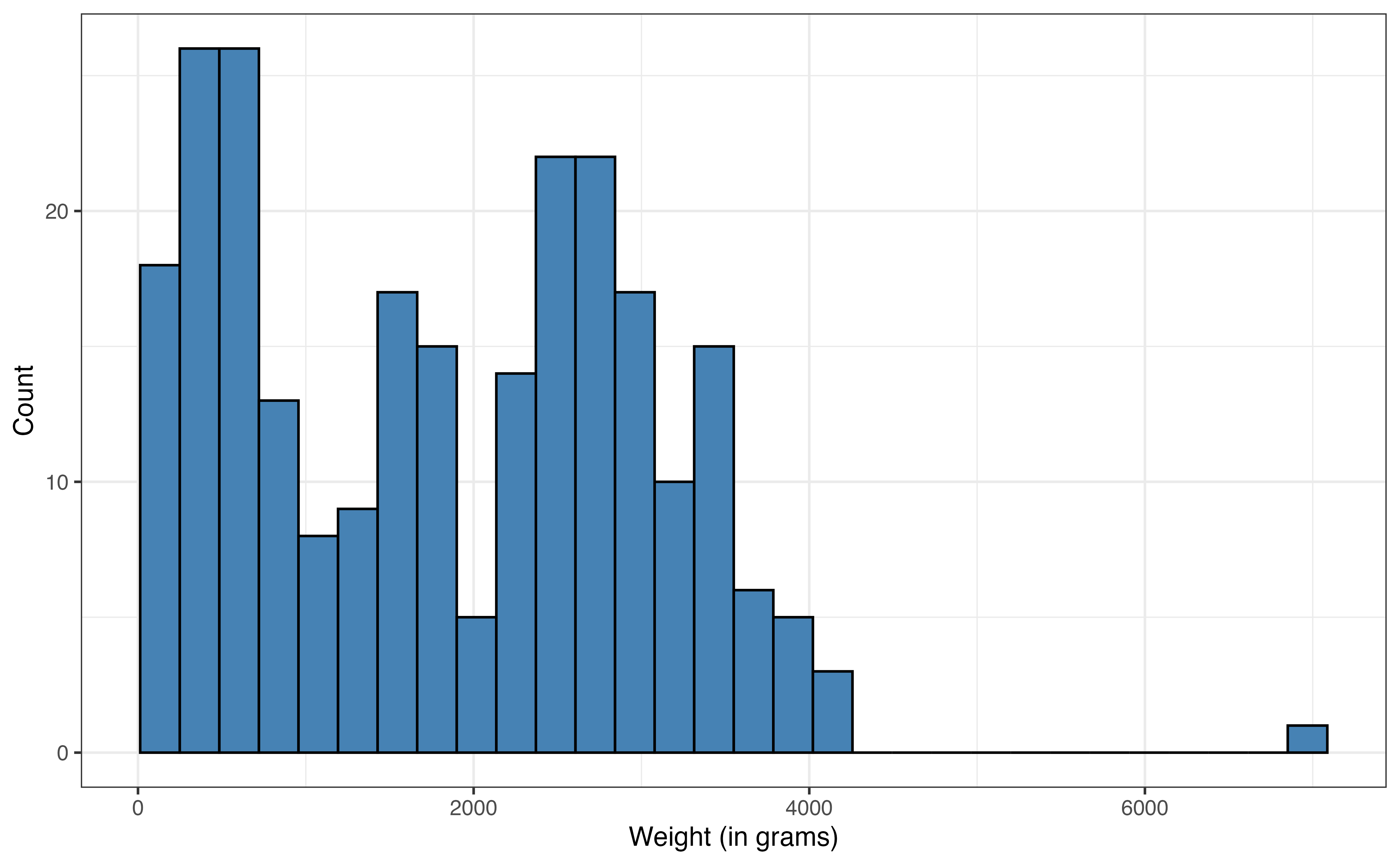
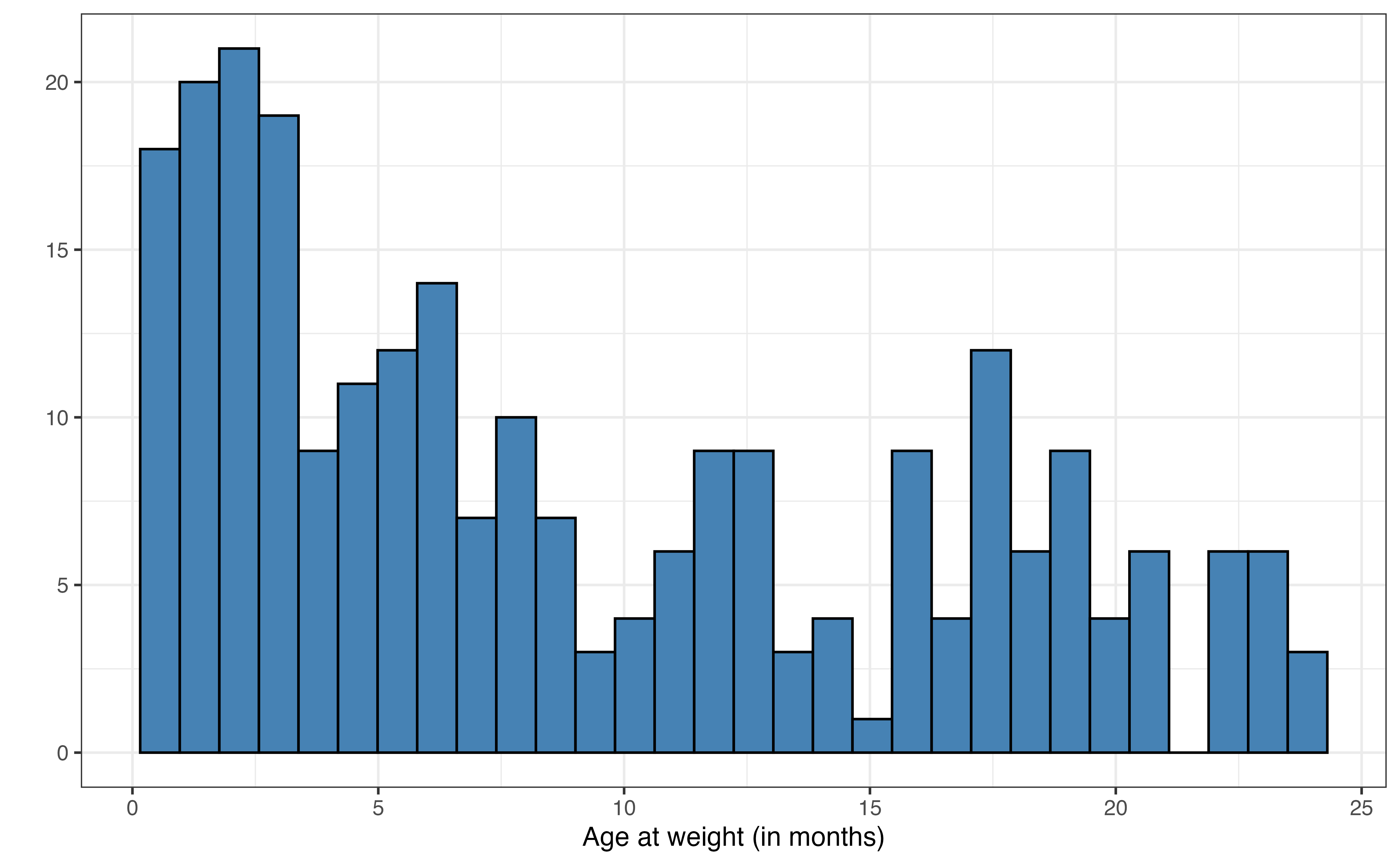
The distribution and summary statistics for the response variable weight are shown in Figure 7.2 and Table 7.1, respectively. The center of the distribution is around the median of 1779.5 grams and the interquartile range (IQR) is 2087 grams. The distribution is bimodal, which may be due to the multiple taxa represented in the data. There is one lemur with a high outlying weight of 6969 grams. We will keep the bimodality and outlier in mind as we proceed with the analysis.

Figure 7.2: Univariate distribution of weight of young lemurs

Table 7.1: Summary statistics for weight

Variable	Mean	SD	Min	Q1	Median (Q2)	Q3	Max	Missing
weight	1839	1190	131	677	1780	2764	6969	0

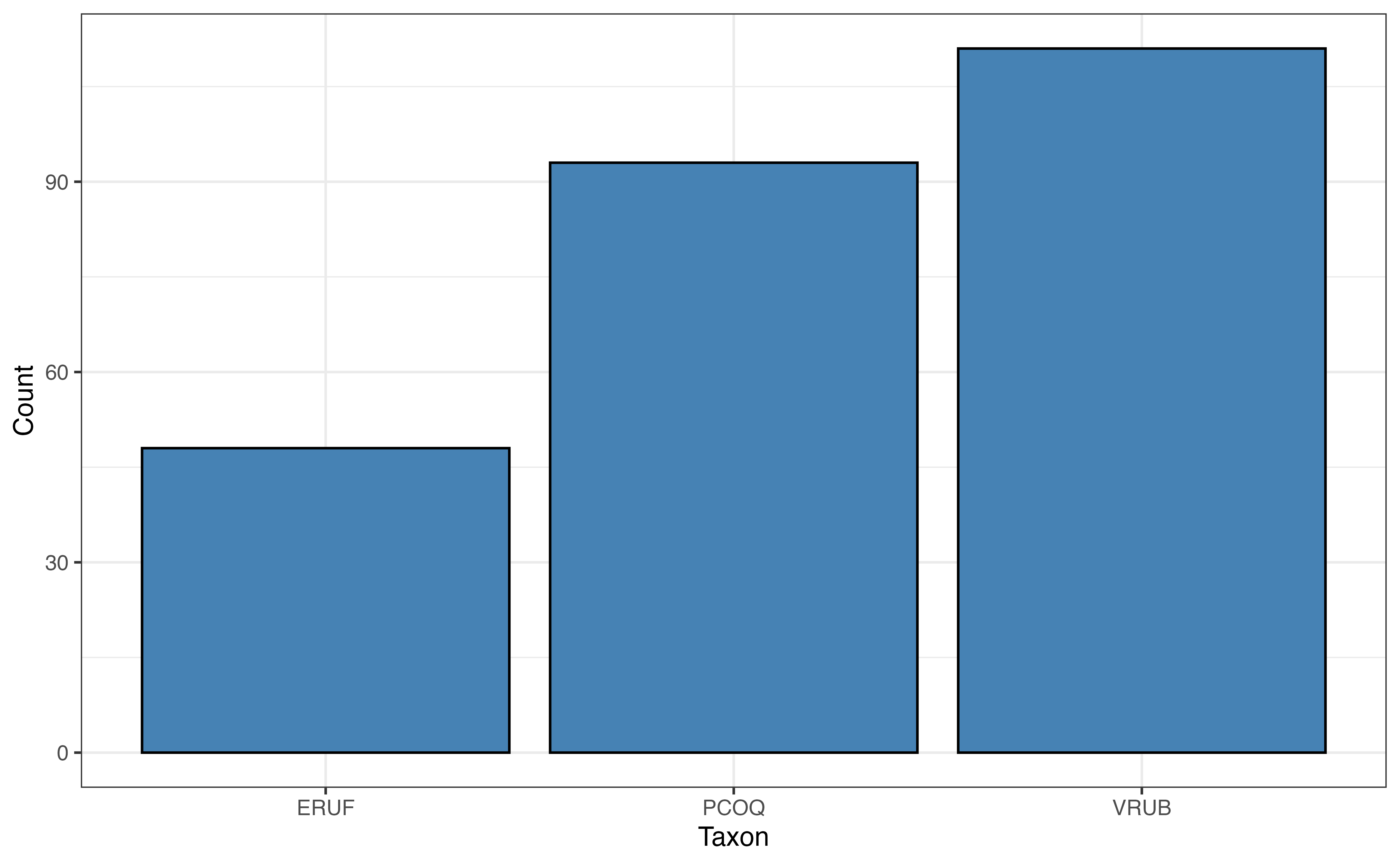
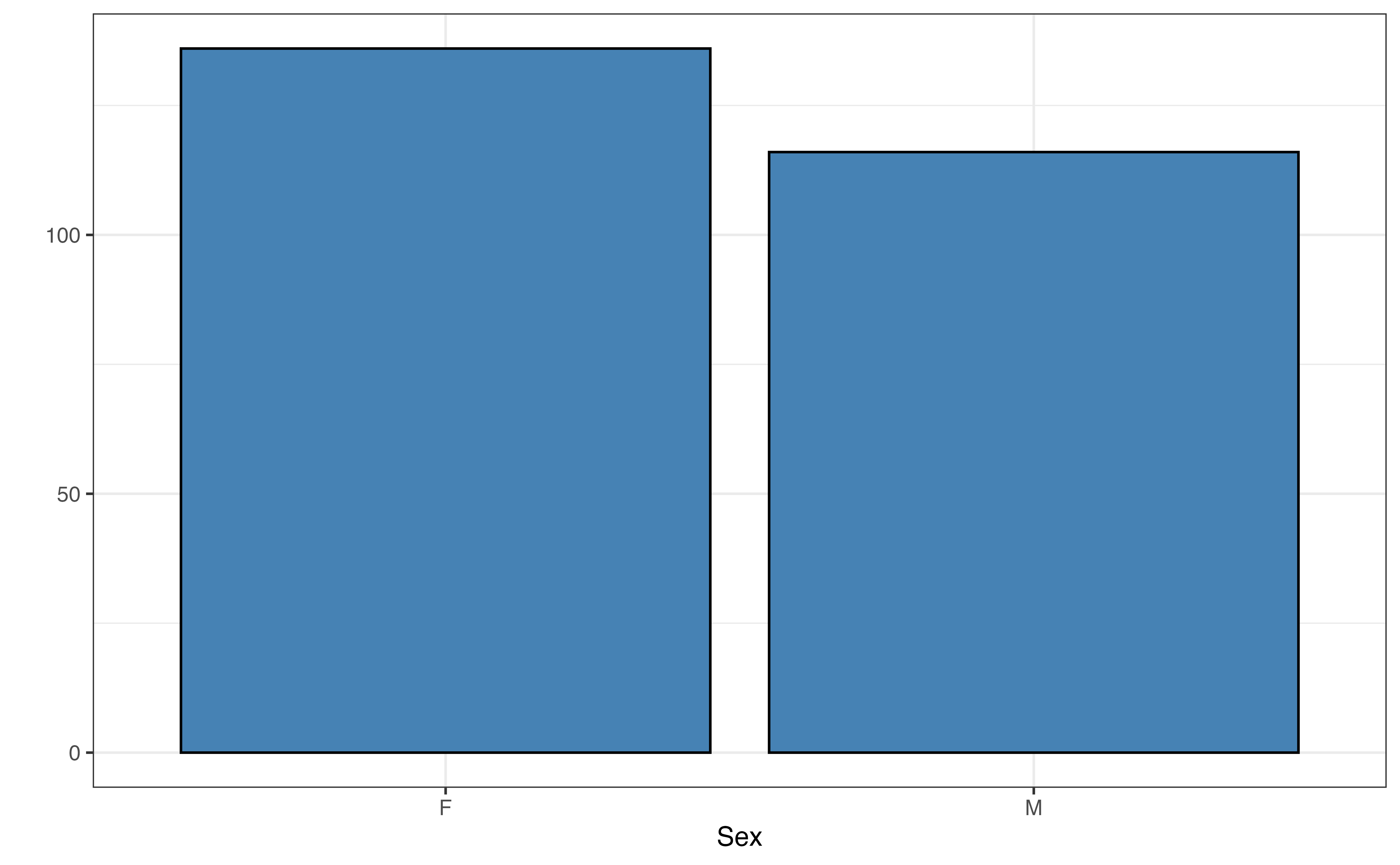
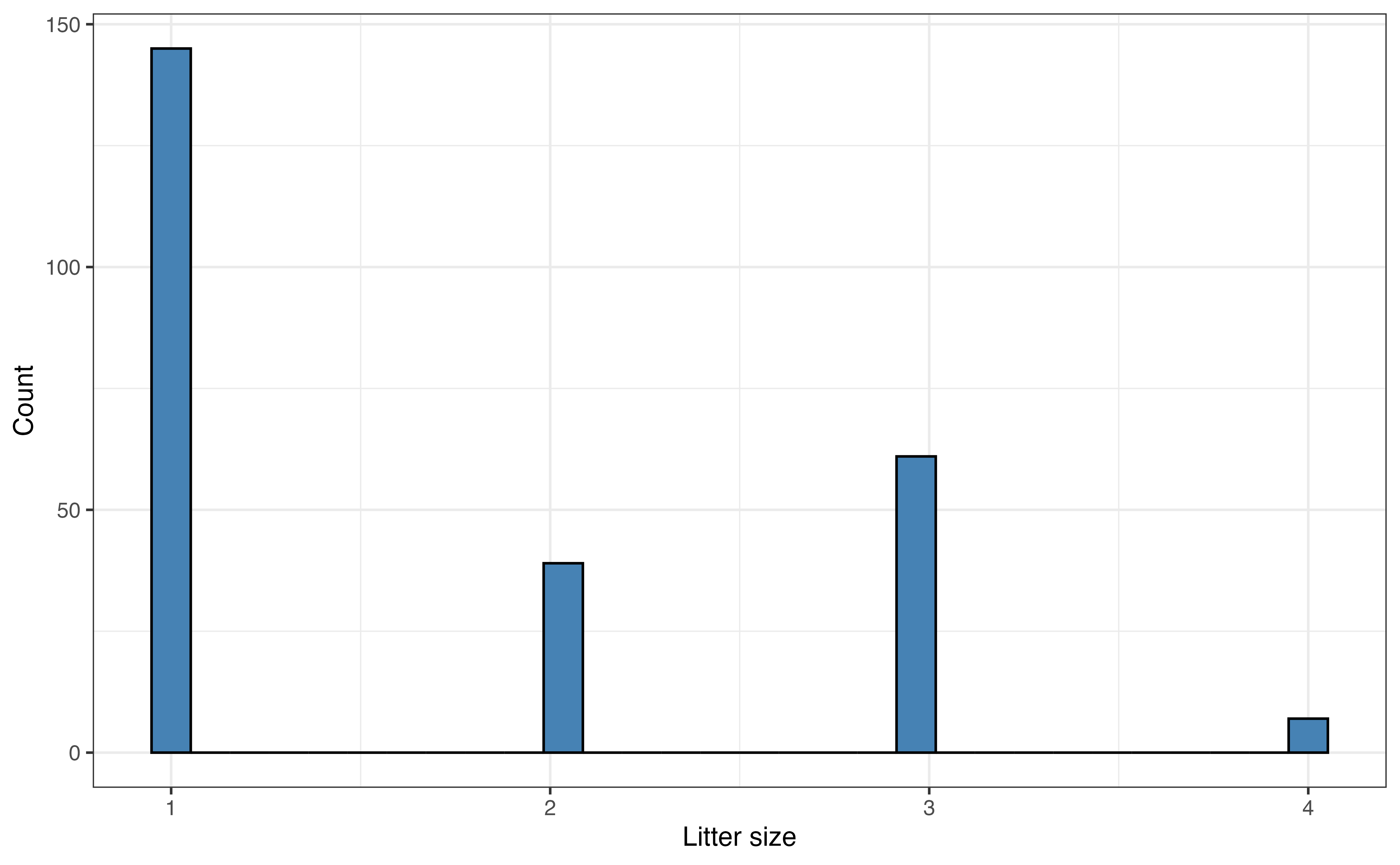
Now let’s look at the distributions of the predictors in this analysis. The visualizations of each variable’s distribution and summary statistics for the quantitative predictors are in Figure 7.3 and Table 7.2, respectively.

(a) age

(b) taxon

(c) sex

(d) litter_size

Figure 7.3: Univariate distributions of predictor variables

Table 7.2: Summary statistics of quantitative predictors

Variable	Mean	SD	Min	Q1	Median (Q2)	Q3	Max	Missing
litter_size	1.7	0.9	1.0	1.0	1.0	3.0	4.0	0
age	9.0	7.0	0.6	2.8	7.1	15.6	23.9	0

The distribution of taxon in Figure 7.3 (b) shows that most lemurs are from the VRUB taxon and the fewest are from the ERUF taxon. The distribution of sex in Figure 7.3 (c) shows a relatively equal distribution, with a small majority of the lemurs being female. Finally, a vast majority of the lemurs were born as the only lemur in their litter as seen in Figure 7.3 (d).

Use the visualizations in Figure 7.3 and summary statistics in Table 7.2 to describe the distribution of age.¹

Now, we conduct bivariate exploratory data analysis, shown in Figure 7.4, to explore the relationship between the response and each of the predictor variables.

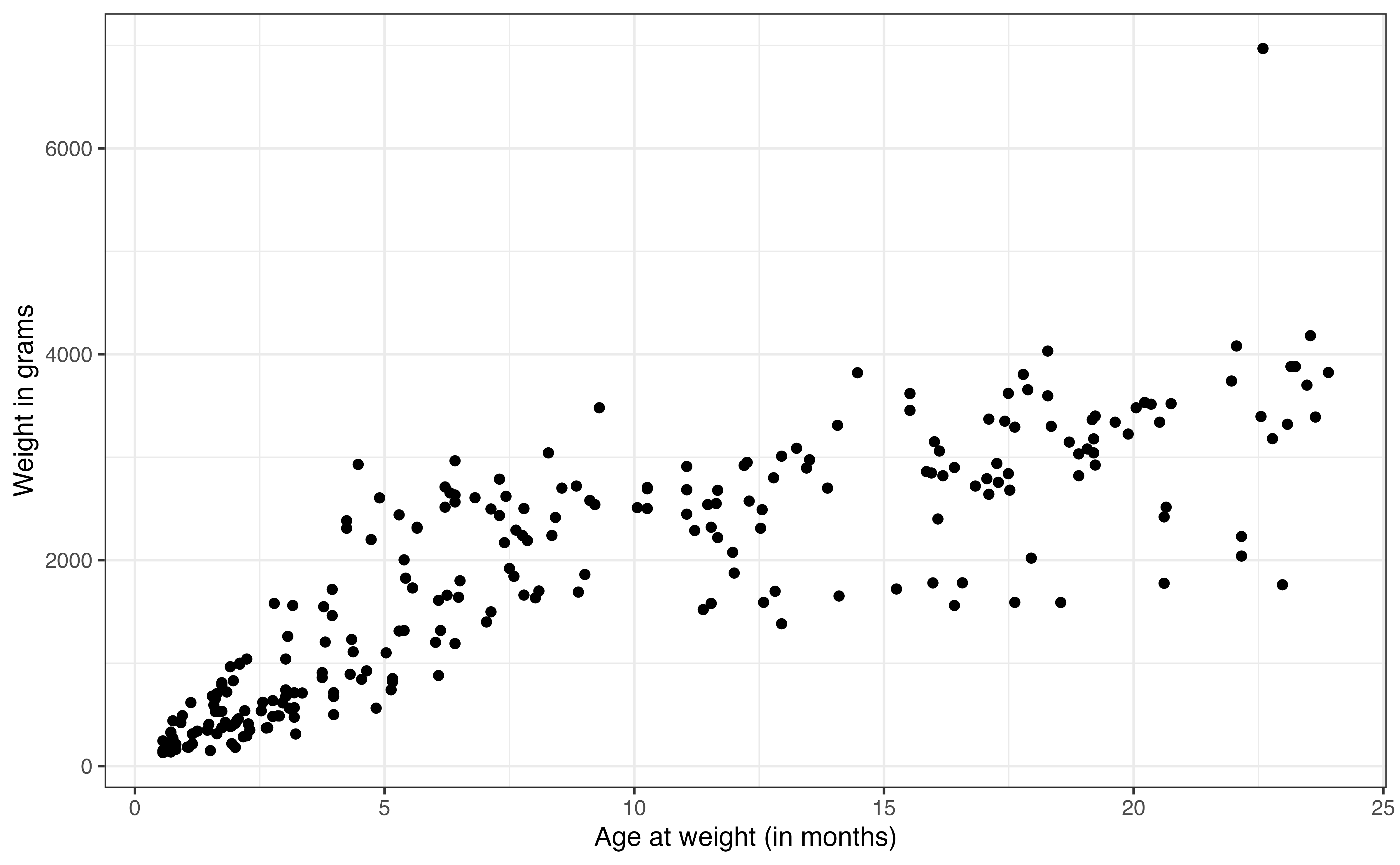
(a) weight vs. age

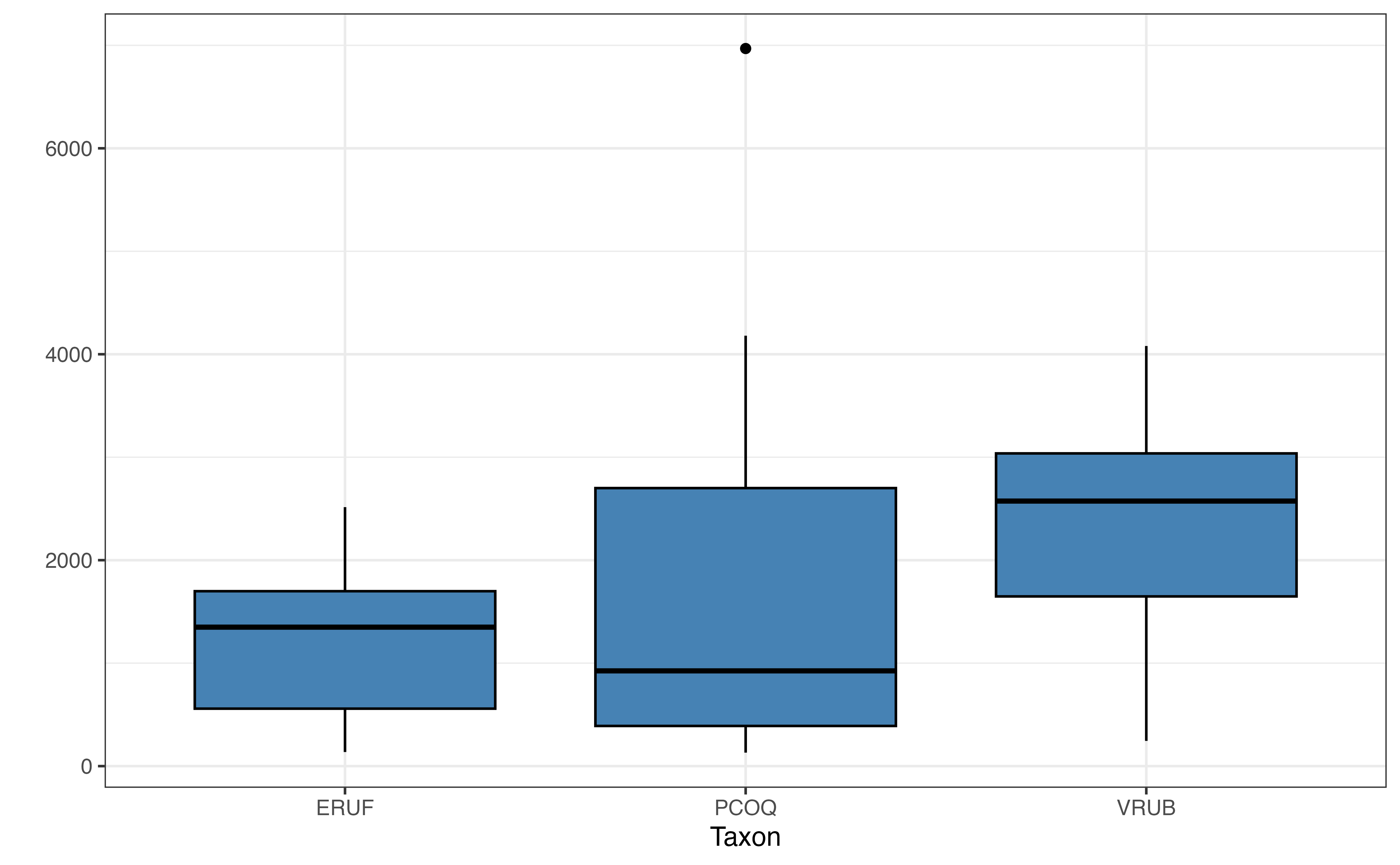
(b) weight vs. taxon

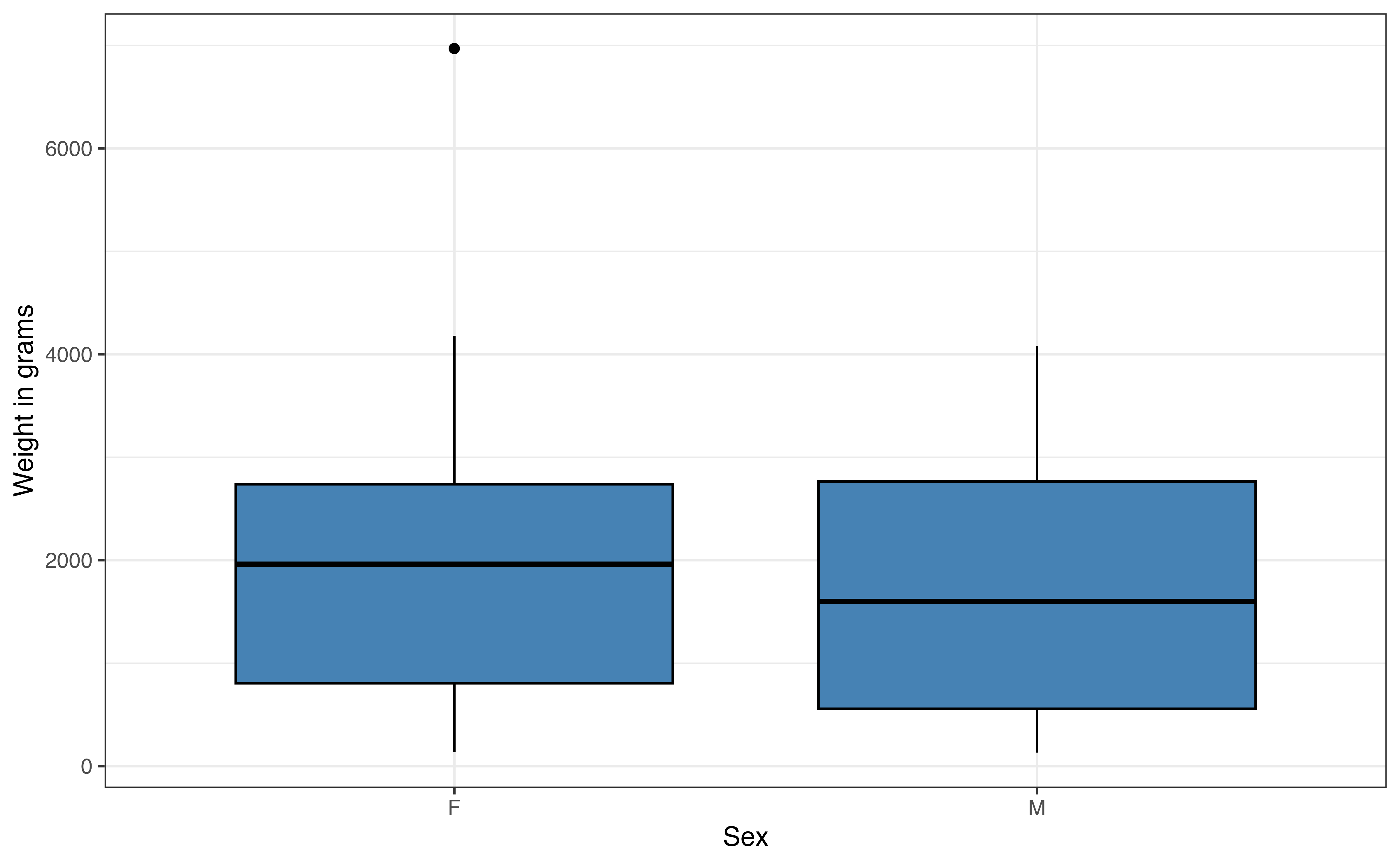
(c) weight vs. sex

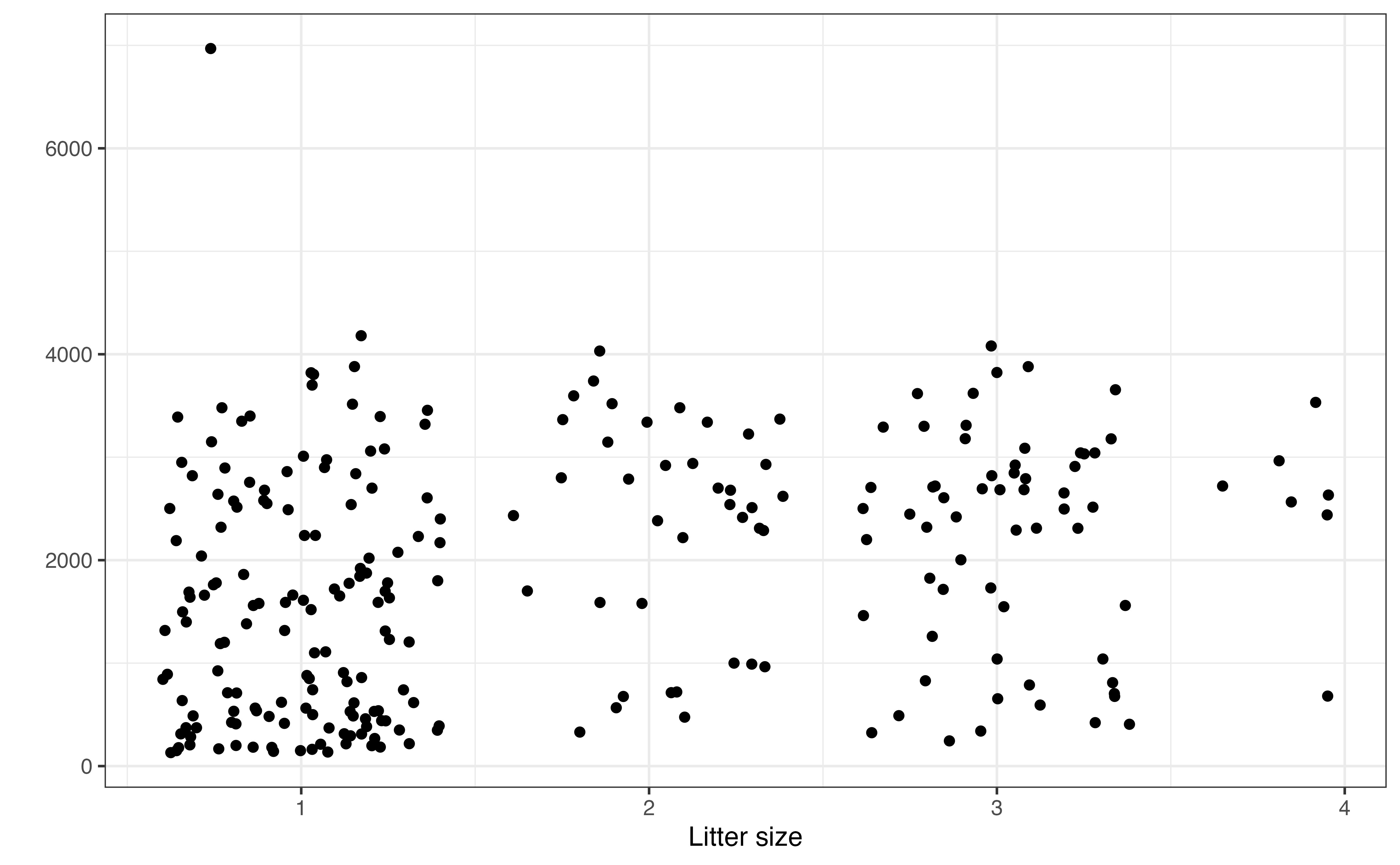
(d) weight vs. litter_size

Figure 7.4: Bivariate exploratory data analysis

From Figure 7.4 (a), we see a strong, positive relationship between age and weight. The relationship looks linear; however, the relationship flattens as age increases. This aligns with what we might expect; lemurs experience fairly rapid growth early on, and then their growth rate slows over time. In Chapter 9, we will introduce transformations that can be applied to the predictor and response variables to account for such trends in the model. For now, we will model the relationship as a constant rate of change between age and weight.

In Figure 7.4 (b), lemurs from the PCOQ taxon have a lower median weight than lemurs from ERUF or VRUB: however, there is a lot of overlap in the distribution of weights of ERUF and PCOQ lemurs. Lemurs in the VRUB taxon have the highest median weight; however, the middle 50% of the distribution overlaps greatly with the distribution for PCOQ lemurs. There is more variability in the weights of PCOQ lemurs compared to ERUF and VRUB, and we see the lemur with the outlier weight is in the PCOQ taxon.

Based on the medians and large overlap in the boxplots in Figure 7.4 (c), there does not appear to be much difference in the weights of male and female lemurs. From this plot, we see the lemur with the high outlying weight is a female.

Figure 7.4 (d) shows the relationship between litter_size and weight. Random noise was added to reduce overlap in the points on the graph. This makes it easier to see the relationship between the two variables. Based on this scatterplot, the relationship between litter_size and weight appears to be positive and relatively weak.

Now that we have a better understanding of the variables in this analysis, we will use a multiple linear regression model to understand how taxon, litter size, age, and sex explains variability in the weight of lemurs. Before looking at the model specific to this data, we will discuss the details of the multiple linear regression model, in general, and to determine if a multiple linear regression model is appropriate for the data.

7.2 Fitting the regression line

In Chapter 4, we introduced simple linear regression to quantify the relationship between a response and a single predictor variable. Using multiple linear regression, we can expand on the regression model to quantify the relationship between a response variable and multiple predictors.

7.2.1 Statistical model for multiple linear regression

Recall from Section 4.3 that the general form of a model for a response variable $Y$ is

$$\begin{array}{}\text{(7.1)}& Y=\text{Model}+\text{Error}\end{array}$$

In the case of simple linear regression, $\text{Model}=f(X)$ where $X$ is the predictor variable used to explain the variability in $Y$. Now we will expand Equation 7.1 to the case in which multiple predictor variables, denoted $\mathbf{X}=X_1,X_2,\dots ,X_p$ are used in combination to explain variability in the response variable $Y$. The values of the response variable $Y$ are generated based on the following equation

$$\begin{array}{}\text{(7.2)}& \begin{array}{rl}Y& =\text{Model}+\text{Error}\\ & =f(\mathbf{X})+ϵ\\ & =f(X_1,X_2,\dots ,X_p)+ϵ\end{array}\end{array}$$

where $p$ represents the number of predictor variables and $ϵ$ is the error term quantifying the amount in which the actual value of $Y$ differs from what is expected from the model $f(X_1,X_2,\dots ,X_p)$.

Equation 7.2 is the general form of the model. As with simple linear regression, we know the form of $f(X_1,X_2,\dots ,X_p)$ when we assume there is a linear relationship between the response and predictor variables. Equation 7.2 can be more specifically written as a multiple linear regression model (MLR) of the form

$$\begin{array}{}\text{(7.3)}& Y={\beta }_0+{\beta }_1{X}_1+{\beta }_2{X}_2+\cdots +{\beta }_p{X}_p+ϵ,ϵ\sim N(0,{\sigma }_{ϵ}^2)\end{array}$$

where $ϵ\sim N(0,{\sigma }_{ϵ}^2)$ indicates the error terms are normally distributed with a mean of 0 and variance ${\sigma }_{ϵ}^2$. Equation 7.3 is the population-level statistical model for multiple linear regression.

Recall from Section 4.3.1, the function $f(X)={\mu }_{Y|X}$ is the expected value (mean) of $Y$ given a value of the predictor $X$. Extending this to multiple linear regression, $f(\mathbf{X})=f(X_1,X_2,\dots ,X_p)$ outputs the expected value of $Y$ for a combination of the predictors. Therefore,

$$\begin{array}{}\text{(7.4)}& {\mu }_{Y|\mathbf{X}}={\mu }_{Y|X_1,X_2,\dots ,X_p}={\beta }_0+{\beta }_1{X}_1+{\beta }_2{X}_2+\cdots +{\beta }_p{X}_p\end{array}$$

Thus, when we fit a multiple linear regression model, the output from the fitted model will be the predicted expected value of the response variable for a given combination of values of the predictor variables.

7.2.2 Evaluating whether MLR is appropriate

Before we move forward with fitting the regression model, we should first ask whether the multiple linear regression model is appropriate or useful for the data. We can ask the same questions we did for simple linear regression; however, now we are considering the relationship between $Y$ and multiple predictor variables rather than a single predictor.

• Will a linear regression model be practically useful? Does quantifying and interpreting the relationship between the variables make sense in this scenario?
• Do the observations in the data represent the population of interest, or are there biases that should be addressed when drawing conclusions from the analysis?
• Would a linear regression model reasonably summarize the relationship between the response and predictor variables?

The last question can be more challenging to answer for multiple linear regression than it was in simple linear regression, because it is difficult to visualize the relationship between three or more variables in the exploratory data analysis. As we saw in Section 7.1.1, we can visualize the relationship between the response and each individual predictor. This can give us some indication of linearity and if there are non-linear trends that need to be taken into account (more on this in Chapter 9). We will primarily rely on the assessment of the model conditions (Section 8.5) to ultimately determine whether a linear model adequately captures the relationship between the response and predictor variables.

7.3 Estimating the coefficients

The predicted value $Y$ for the $i^{th}$ observation output from the estimated multiple linear regression is shown in Equation 7.5 is

$$\begin{array}{}\text{(7.5)}& {\hat{y}}_i={\hat{\mu }}_{y_i|x_{i1},x_{i2},\dots ,x_{ip}}={\hat{\beta }}_0+{\hat{\beta }}_1{x}_{i1}+{\hat{\beta }}_2{x}_{i2}+\cdots +{\hat{\beta }}_p{x}_{ip}\end{array}$$

The error term for the $i^{th}$ observation, ${ϵ}_i$, is estimated by calculating the residuals as before, $e_i=y_i-{\hat{y}}_i$, the difference between what is observed in the data and what is expected from Equation 7.5. As with simple linear regression in Section 4.4, the coefficients are estimated using least-squares, finding ${\hat{\beta }}_0,{\hat{\beta }}_1,\dots ,{\hat{\beta }}_p$ that minimize the sum of square residuals shown in Equation 7.6

$$\begin{array}{}\text{(7.6)}& \sum _{i=1}^n{e}_i^2=\sum _{i=1}^n(y_i-{\hat{y}}_i{)}^2=\sum _{i=1}^n(y_i-[{\beta }_0+{\beta }_1{x}_{i1}+\cdots +{\beta }_p{x}_{ip}]{)}^2\end{array}$$

7.3.1 (Optional) Matrix notation for multiple linear regression

The calculus required to find the values that minimize Equation 7.6 can become quite cumbersome, particularly if there are a lot of predictor variables. We can instead think of Equation 7.3 and Equation 7.5 in terms of matrices and utilize linear algebra and matrix calculus to compute the estimated coefficients. Suppose there are $n$ observations and $p$ predictors, then

$$\mathbf{Y}=\left[\begin{array}{c}{y}_1\\ y_2\\ ⋮\\ y_n\end{array}\right]\mathbf{X}=\left[\begin{array}{ccccc}1& x_{11}& x_{12}& \dots & x_{1p}\\ 1& x_{21}& x_{22}& \dots & x_{2p}\\ ⋮& ⋮& \ddots & ⋮& ⋮\\ 1& x_{n1}& x_{n2}& \dots & x_{np}\end{array}\right]$$

where $\mathbf{Y}$ is an $n\times 1$ vector of the values of the response, and $\mathbf{X}$ is an $n\times (p+1)$ matrix called the design matrix. The first column of $\mathbf{X}$ is a vector of 1’s that correspond to the intercept ${\beta }_0$. The remaining columns are the observed values for each predictor variable. For example, the row $\left[\begin{array}{ccccc}1& x_{11}& x_{12}& \dots & x_{1p}\end{array}\right]$ contains the observed values for the first observation, and

the column ${\left[\begin{array}{cccc}{x}_{11}& x_{21}& \dots & x_{n1}\end{array}\right]}^{\mathsf{T}}$ is the column of observed values for predictor $X_1$.

Additionally, let

$$\mathit{\beta }=\left[\begin{array}{c}{\beta }_0\\ {\beta }_1\\ ⋮\\ {\beta }_p\end{array}\right]\mathit{ϵ}=\left[\begin{array}{c}{ϵ}_1\\ {ϵ}_2\\ ⋮\\ {ϵ}_n\end{array}\right]$$

such that $\mathit{\beta }$ is a $(p+1)\times 1$ vector of the model coefficients and $\mathit{ϵ}$ is an $n\times 1$ vector of the error terms. Equation 7.3 written in matrix notation is

$$\underset{\mathbf{Y}}{\underbrace{\left[\begin{array}{c}{y}_1\\ y_2\\ ⋮\\ y_n\end{array}\right]}}=\underset{\mathbf{X}}{\underbrace{\left[\begin{array}{ccccc}1& x_{11}& x_{12}& \dots & x_{1p}\\ 1& x_{21}& x_{22}& \dots & x_{2p}\\ ⋮& ⋮& \ddots & ⋮\\ 1& x_{n1}& x_{n2}& \dots & x_{np}\end{array}\right]}}\underset{\mathit{\beta }}{\underbrace{\left[\begin{array}{c}{\beta }_0\\ {\beta }_1\\ ⋮\\ {\beta }_p\end{array}\right]}}+\underset{\mathit{ϵ}}{\underbrace{\left[\begin{array}{c}{ϵ}_1\\ {ϵ}_2\\ ⋮\\ {ϵ}_n\end{array}\right]}}$$

$$\begin{array}{}\text{(7.7)}& \mathbf{Y}=\mathbf{X}\mathit{\beta }+\mathit{ϵ}\end{array}$$

Similarly, Equation 7.5 in matrix notation is

$$\hat{\mathbf{Y}}=\mathbf{X}\hat{\mathit{\beta }}$$

Applying the rules of linear algebra and matrix calculus, we find that the estimated coefficients ${\hat{\beta }}_0,{\hat{\beta }}_1,\dots ,{\hat{\beta }}_p$ can be found using Equation 7.8

$$\begin{array}{}\text{(7.8)}& \hat{\mathit{\beta }}=({\mathbf{X}}^{\mathsf{T}}\mathbf{X}{)}^{-1}{\mathbf{X}}^{\mathsf{T}}\mathbf{Y}\end{array}$$

Details for using the matrix form of the model to find $\hat{\mathit{\beta }}$ in Equation 7.8 are in Section A.3.

Matrix form of simple linear regression

The design matrix $\mathbf{X}$ and the vector of coefficients $\mathit{\beta }$ are indexed by the number of predictors $p$. The number of predictors can be any value between 1 and $n$, the number of observations². Therefore, the linear regression computations in matrix form apply to simple linear regression as well.

One way to practice using the matrix representation of the model is to compare the results from simple linear regression in Section 4.4 to the results using matrix notation.

7.4 Interpreting model coefficients

The fitted model for explaining variability in the weight of young lemurs is in Table 7.3. We refer to this model as we interpret the model coefficients.

Table 7.3: Output of model using various characteristics to explain variability in weight of young lemurs

term	estimate	std.error	statistic	p.value
(Intercept)	43.8	121.72	0.360	0.719
age	136.9	4.86	28.182	0.000
sexM	-88.8	68.00	-1.306	0.193
taxonPCOQ	471.7	95.43	4.943	0.000
taxonVRUB	1037.3	133.91	7.747	0.000
litter_size	-19.6	65.80	-0.298	0.766

7.4.1 Interpreting coefficients of quantitative predictors

The interpretation for coefficients of quantitative predictors is similar to the interpretation in simple linear regression in Section 4.5. Given a quantitative predictor $x_j$, its model coefficient ${\beta }_j$ is the slope describing the relationship between $x_j$ and the response variable, after accounting for the other predictors in the model. For example, the coefficient for age in Table 7.3 is 136.903. Let’s compare this to the coefficient from a simple linear regression model using age shown in Table 7.4.

Table 7.4: Simple linear regression model of weight versus age

term	estimate	std.error	statistic	p.value
(Intercept)	555	67.31	8.25	0
age	142	5.88	24.12	0

In the model in Table 7.4 that only uses age to predict weight, the weight is expected to increase by 141.892 grams, on average for each month increase in age. If we also take into account sex, taxon, and litter size in addition to age, then the weight is expected to increase by 136.903 grams, on average, as age increases by one month. This means some of the change in weight as age increases in Table 7.4 can be explained by the other predictors in Table 7.3.

We write the interpretation of the coefficients in a multiple linear regression models in a way that indicates there are other variables being taken into account in the model. There are two commonly used ways to word this. The first is by interpreting the coefficient ${\beta }_j$ as the expected change in the response variable when $x_j$ increases by one unit, adjusting for all other predictors in the model. This interpretation means that once we have taken into account the relationship between all the other predictors and the response variable, then we have isolated the effect of the predictor $x_j$ and thus can explain the relationship between the response variable and the predictor $x_j$. The second way is to specify that all other predictors are held constant. This means that if have two observations with the same values for all other predictors, then we see how the value of the response is expected to change between these two observations as $x_j$ changes.

Let’s apply this to interpret age in the model in Table 7.3. The following are two acceptable forms of the interpretation:

For each additional month in a young lemur’s age, their weight is expected to be greater by 136.903 grams, on average, adjusting for taxon, sex, and litter size.

For each additional month in a young lemur’s age, their weight is expected to be greater by 136.903 grams, on average, holding taxon, sex, and litter size constant.

The phrase “holding all else constant” stems from the fact that multiple linear regression is conducted assuming the predictors are independent. Some argue, however, that it is not feasible for the predictors to be completely independent in practice, so the phrasing “adjusting for all other predictors” may better represent the model in practice. We will use both forms of the interpretation throughout the book. We talk more about more the relationship between the predictors in Chapter 8.

Interpret the coefficient litter_size in the context of the data.

Recall from Section 4.5, “in the context of the data” means

• using the variable names or meaningful descriptions of the variables,
• including the units in the interpretation, and
• Indicating the population for which this model applies.³

7.4.2 Interpreting coefficients of categorical predictors

When categorical predictors are included in a model, we need a way to transform the levels (or categories) of the predictor into quantitative information that can be used in the regression calculations. To do so, indicator variables are created for each level of the categorical predictor. We then use these indicator variables in the regression model.

Suppose we have a categorical variable that has $k$ levels. We define $k$ indicator variables, one for each level, such that the indicator takes the value $1$ if the observation belongs to the particular level and $0$ if the observation does not belong to the particular level. Let’s take a look at the variable taxon in the lemurs data.

The variable taxon has three levels, ERUF, PCOQ, and VRUB, so we create three indicator variables. We will call these indicators taxonERUF, taxonPCOQ, and taxonVRUB. Table 7.5, shows the number of observation at each level of the original variable taxon and the number of observations that take values 1 or 0 for each indicator variable.

Table 7.5: Indicator variables for taxon

taxon	taxonERUF	taxonPCOQ	taxonVRUB	n
ERUF	1	0	0	48
PCOQ	0	1	0	93
VRUB	0	0	1	111

Now we are ready to use the indicator variables in the model. In Table 7.3, we see there are only two indicator variables (not three) for taxon in the model. When there are $k$ levels of a categorical predictor, there are $k-1$ indicator variables for the categorical predictor included in the model. The level that does not have an indicator variable in the model is called the baseline level (this is also known as the reference level). Thus, the interpretation of the coefficients for indicator variables describe how much the expected response for a given level is expected to differ, on average, compared to the expected response at the baseline level, after adjusting for the other predictors in the model.

Let’s take a look at the indicator variables for taxon in Table 7.3. The baseline level is “ERUF”, the taxon that is not represented by an indicator variable in the model. Therefore, the interpretations of the coefficients for taxonPCOQ and taxonVRUB will be how the weights for young lemurs in those taxa are expected to differ, on average, to the weight for lemurs in the ERUF taxon, after adjusting for age, sex, and litter size.

The coefficient for the PCOQ taxon is ${\hat{\beta }}_{PCOQ}=$ 471.715. This means that the expected weight is 471.715 grams greater, on average, for lemurs in the PCOQ taxon compared to the expected weight for lemurs in the ERUF taxon, holding age, sex, and litter size constant.

The coefficient for the VRUB taxon is ${\hat{\beta }}_{VRUB}=$ 1037.323. This means that the expected weight is 1037.323 grams greater, on average, for lemurs in the VRUB taxon compared to the expected weight for lemurs in the ERUF taxon, holding age, sex, and litter size constant.

The code in ?sec-mlr-estimate-R shows that we only need to put the name of the categorical predictor into the lm function for fitting the model. R (and other statistical software) will create indicator variables behind the scenes and selects the baseline level as the following:

• If the categorical predictor is nominal (it has no inherent order like taxon), then R chooses the first level alphabetically to be the baseline. R made ERUF the baseline level for taxon, because it is first alphabetically in the list of ERUF, PCOQ, and VRUB.

• If the categorical predictor is ordinal (there is some order imposed), then R chooses the lowest level to be the baseline.

As the data scientists, we can determine which level we would like to be the baseline level if neither of these approaches align well with the data. To do so, use functions to impose an ordering with the desired baseline as the first level.

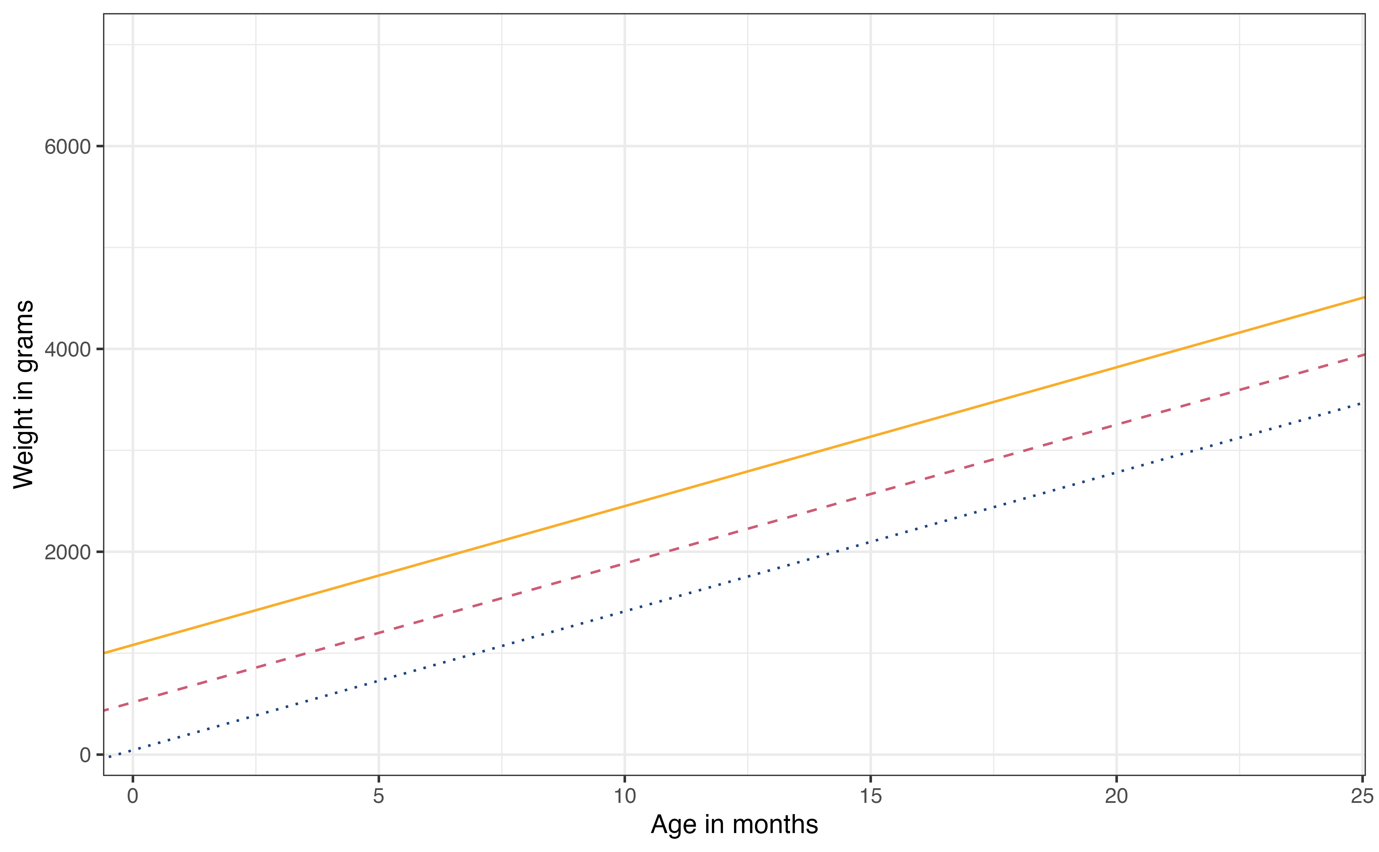
Indicator variables in the model describe how much the intercept of the model shifts based on the levels of the categorical variable. The intercept term in the model is the intercept associated with the baseline level for the categorical predictor. This means the intercepts for taxon are the following:

• ERUF: 43.844

• PCOQ: 515.559 (43.844 + 471.715)

• VRUB: 1081.167 (43.844 + 1037.323 )

This shift in the intercept is visually represented in the scatterplot of age versus weight by taxon in Figure 7.5.

Figure 7.5: Different intercepts for each taxon. Purple dotted line = ERUF, Pink dashed line = PCOQ, Yellow sold line = VRUF

The other categorical predictor in the model in Table 7.3 is sex.

• What is the baseline level for sex?
• Interpret the coefficient of sex in the context of the data.
• What is the intercept for female lemurs? For male lemurs?⁴

7.4.3 Interpreting the intercept

As with simple linear regression, the intercept is the expected value of the response when all predictors in the model equal 0. Let’s take a look at what this means for our model in Table 7.3. The intercept is at the point such that

• age = 0: The lemur is 0 months old at the time of the weight
• sexM = 0: The lemur is female.
• taxonPCOQ = 0 and taxonVRUB = 0: The lemur is from the ERUF taxon. (See Table 7.5 to confirm this)
• litter_size = 0: There were 0 lemurs in the litter size in which the lemurs born. (Note that this is not a possible in the data set).

Based on the model, the expected weight for such lemurs is about 43.844 grams.

Putting this together in narrative form, we have

The expected weight for female lemurs from the ERUF taxon who are 0 months old at the time of weight and were born into a litter with 0 lemurs is about 43.844 grams.

As in SLR, we need the intercept to get the least-squares model. The intercept, however, does not always have a meaningful interpretation in practice. Therefore, as with simple linear regression, the intercept has a meaningful interpretation when the following are true:

1. The scenario described by all the predictors in the model being at or near zero is plausible in practice.

2. The data used to fit the model includes observations in which all the predictors are at or near zero.

Based on these criteria, do you think the interpretation of the intercept is meaningful for the lemurs data? Why or why not?⁵

7.5 Prediction

The same process is used to predict for multiple linear regression as the one introduced in Section 4.6 for simple linear regression. Now that there are two or more predictor variables, we need to input a value for every predictor variable.

For example, suppose we wish to use the model in Table 7.3 to compute the predicted weight for a 10-month old male lemur in the VRUB taxon who was born into a litter of 4 lemurs. We compute this value by plugging in the value for the new observation into the model equation as shown in Equation 7.9.

$$\begin{array}{}\text{(7.9)}& \begin{array}{rl}\widehat{\text{weight\_g}}& =43.844\\ & +136.903\times 10\\ & -88.838\times 1\\ & +471.715\times 0\\ & +1037.323\times 1\\ & -19.607\times 4\\ & =2282.931\end{array}\end{array}$$

Use the equation in Table 7.3 to compute the predicted value for a 14-month old female lemur in the ERUF taxon who was born into a litter of 2 lemurs. It should match the predicted value shown it the output above.⁶

It is important to avoid extrapolation when making predictions using a multiple linear regression model. This can sometimes to be challenging to assess, as extrapolation might occur both in terms of a single predictor variable being far outside the range in the data but also in terms of a combination of predictors being outside the general patterns observed in the data. When working with real-world data, we can consider if the combination of predictor values can be realistically observed in the population being studied. If that is the case, and the data are representative of the population, then the combination of values if likely to be within the trend represented in the data.

One more consideration for prediction is that we expect there to be some uncertainty in the predicted values, because they are computed based on a model fit using sample data.

7.6 Centered and standardized predictors

7.6.1 Centered quantitative predictors

We need an intercept to fit the least-squares regression model, but it may not have a meaningful interpretation as seen in the example in Section 7.4.3. This is usually because it is not meaningful or realistic for a quantitative variable to take values at or near zero. One way to remedy this is to shift the distribution of one or more quantitative predictors, such that it would be feasible for the shifted predictors to take values near zero. This process is called centering.

Centering a predictor means to shift every observation of that predictor by a single constant, denoted $C$. For example, given a predictor $X$, then the centered version of the predictor is $X_{cent}=X-C$. Thus when $X_{cent}$ is a predictor in the model (instead of $X$), then the intercept is now the expected response when $X_{cent}=X-C=0$, which occurs when $X=C$.

In the previous section, we determined that it is not possible for the litter size to be 0, because the litter size includes the observed lemur. Therefore, we can use centering to create a new variable litter_size_cent by shifting litter_size by 1, so that litter_size_cent = 0 means litter_size = 1 . Though it is not always the case, the newly centered variable litter_size_cent has a new meaningful interpretation. It is the number of siblings of in the litter. Putting this together, litter_size_cent = 0 means the lemur was born into a litter with no siblings.

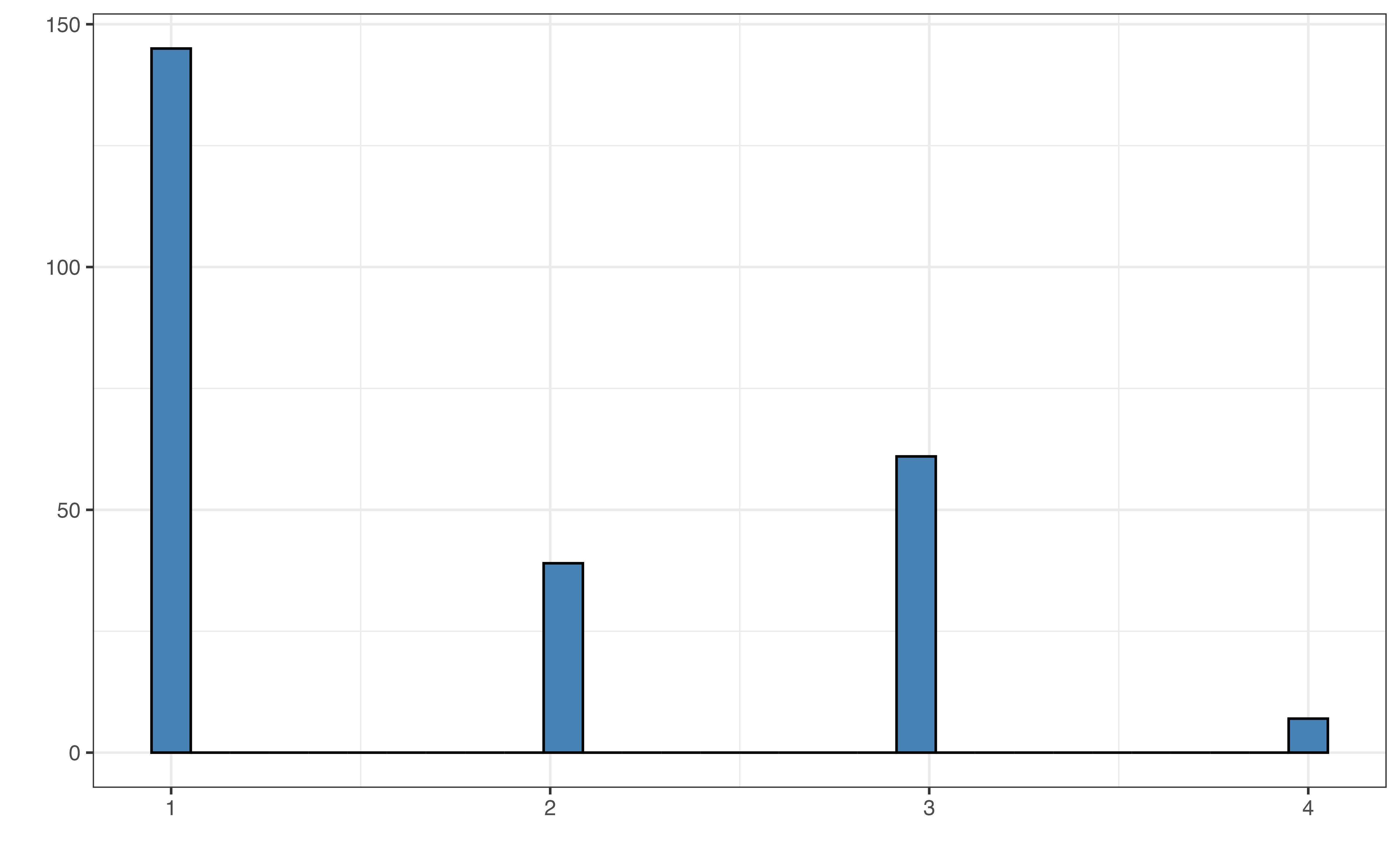
Because this centered variable has its own meaningful interpretation, we will rename the variable to more clearly indicate what this variable is measuring. We call the centered variable litter_size_siblings and use this name for the centered variable moving forward. The distributions of the original and centered variables are shown in Figure 7.6 and Table 7.6.

(a) Distribution of litter_size

(b) Distribution of litter_size_siblings

Figure 7.6: Original versus centered values of litter_size

Table 7.6: Distributions of litter_size vs litter_size_siblings

Variable	Mean	SD	Min	Q1	Median (Q2)	Q3	Max
litter_size	1.7	0.9	1	1	1	3	4
litter_size_siblings	0.7	0.9	0	0	0	2	3

From Figure 7.6 and Table 7.6, we see that the only statistics that have changed are those about location (e.g., $Q1$, $Q3$, min, max) and those related the center (mean and median). The shape of the distribution and statistics regarding the spread (standard deviation and IQR) have remained the same after centering. By centering the variable we have essentially moved the distribution along the number line by some constant amount.

Figure 7.7 shows the relationship between weight versus the original and centered values of litter_size. Both plots have the same slope, illustrating that the slope of the relationship between the predictor and response has not changed by centering. All that has changed is what in means to be “zero”, what observations whose expected response is at the intercept. This is illustrated by the different intercepts for the models shown in the two plots.

(a) weight versus litter_size

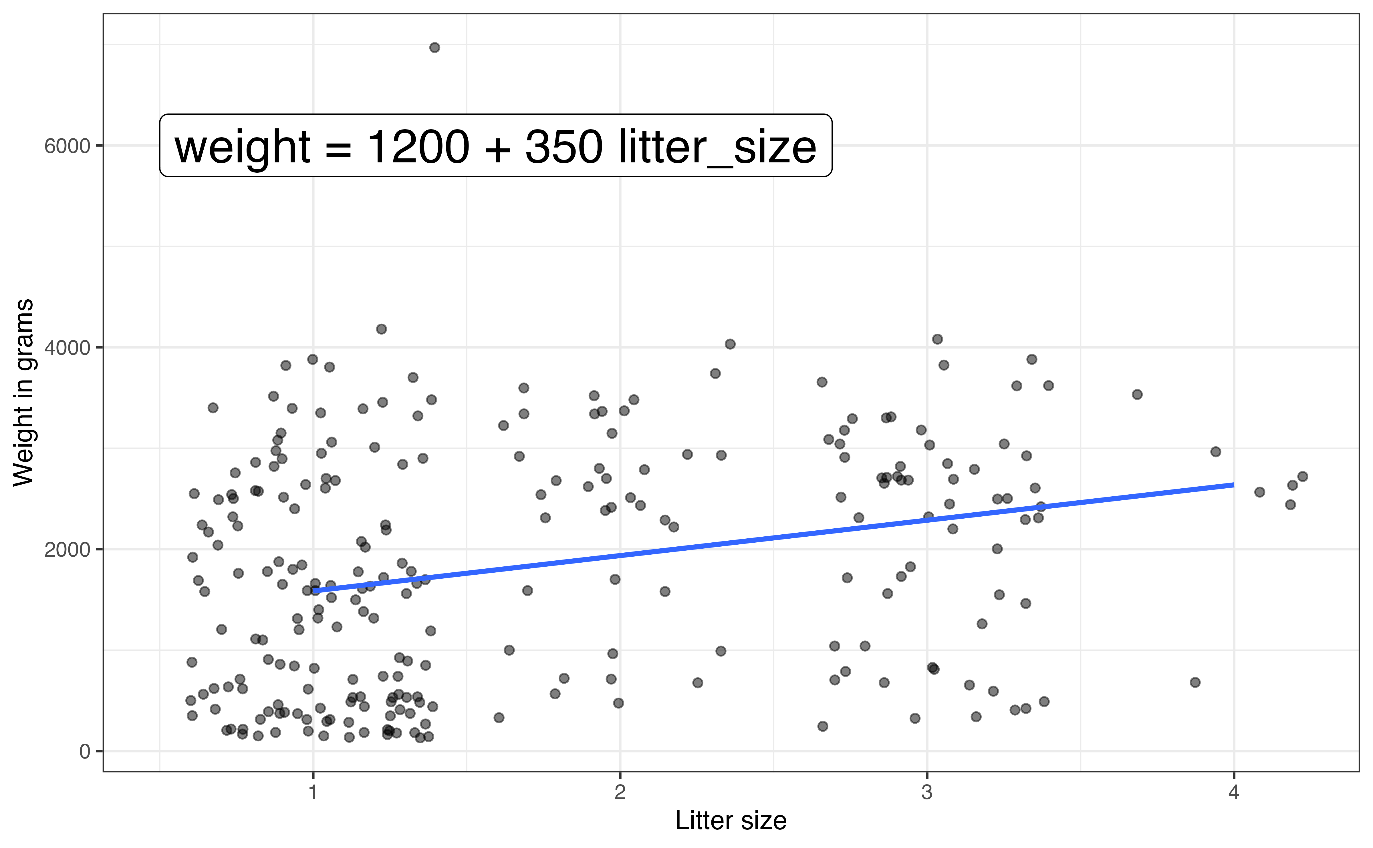
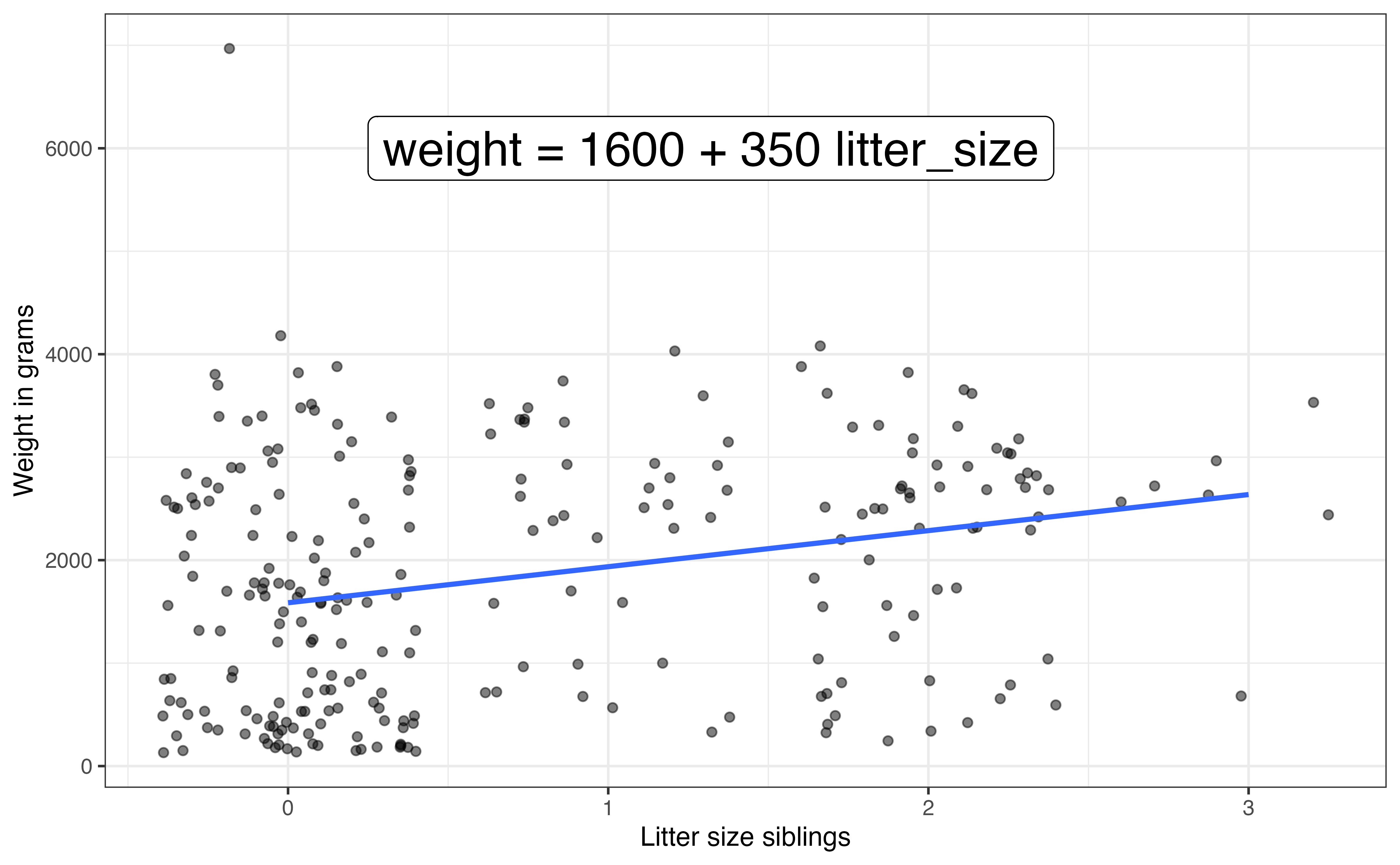
(b) weight versus litter_size_siblings

Figure 7.7: Weight versus original and centered values of litter size

A commonly used type of centering is mean-centering, in which $C=\overline{X}$, meaning a quantitative predictor is shifted by its mean. Let’s mean-center age, so that the intercept does not represent lemurs who are 0 months old, but rather lemurs are who are the mean age in the data set.

$$\text{age\_cent}=\text{age}-\text{mean(age)}$$

Table 7.7 is a table of the summary statistics for the age and age_cent. As before, the location statistics have changed but the variability is the same.

Table 7.7: Distributions of age and age_cent

Variable	Mean	SD	Min	Q1	Median (Q2)	Q3	Max
age	9	7	0.6	2.8	7.1	15.6	23.9
age_cent	0	7	-8.5	-6.3	-2.0	6.6	14.9

Note that we do not mean-center the categorical predictors sex and taxon, because there is already a meaningful interpretation for the indicator variables for these predictors being equal to 0, and there is not a realistic notion of the “average taxon” or “average sex”. Unlike the categorical predictors, we could mean-center litter_size as well.; however, we created the new variable litter_size_siblings by shifting by 1.

.

The output for the model with age_cent and litter_size_siblings, the centered and litter size respectively, is is in Table 7.8 .

Table 7.8: Model for lemurs data with centered quantitative predictors

term	estimate	std.error	statistic	p.value
(Intercept)	1263.2	81.59	15.482	0.000
age_cent	136.9	4.86	28.182	0.000
sexM	-88.8	68.00	-1.306	0.193
taxonPCOQ	471.7	95.43	4.943	0.000
taxonVRUB	1037.3	133.91	7.747	0.000
litter_size_siblings	-19.6	65.80	-0.298	0.766

A comparison of the model coefficients from the original model and the model with the mean-centered values for the quantitative predictors is shown in Table 7.9. Let’s consider in what ways the two models are the same and in what ways they are different.

Table 7.9: Model coefficients for original model and model with centered quantitative predictors

Term	Original	Centered
(Intercept)	43.8	1263.2
age	136.9	136.9
sexM	-88.8	-88.8
taxonPCOQ	471.7	471.7
taxonVRUB	1037.3	1037.3
litter_size	-19.6	-19.6

The only term that changed between the two models is the intercept; the coefficients for all other predictors remained the same. This shows that centering one or more quantitative predictors, by shifting by the mean or some other constant, does not change the relationships between the predictor variables with the response variable. With this in mind, let’s interpret the intercept for the model with the centered variables.

As before, the intercept is the expected weight when all the predictors are equal to 0. Thus, using the model in Table 7.8, the intercept is the expected weight when

• age_cent = 0: The lemur is the mean age in the sample, 9.05 months old.

• sexM = 0: The lemur is female.

• taxonPCOQ = 0 and taxonVRUB = 0: The lemur is from the ERUF taxon.

• litter_size_siblings = 0: The lemur was born into a litter with 0 other lemurs (litter_size = 1).

The interpretation of the intercept in narrative form when the quantitative predictors are centered is

The expected weight for female lemurs from the ERUF taxon who are 9.05 months old and were born into a litter with no siblings is about 1263.178 grams.

Because the coefficients for the other predictors are the same, the interpretations for these predictors are the same as in Section 7.4.1 and Section 7.4.2.

7.6.2 Standardized quantitative predictors

Thus far, we have interpreted the coefficients to understand the relationship between the response and each predictor variable. Sometimes, however, the primary objective of the analysis may be less focused on interpretation and more focused on identifying which predictors are most important in understanding variability in the response variable. When that is the case, we can fit a model using standardized values of the quantitative predictors.

Standardizing a variable is shifting every observation of that variable by its mean (as in mean-centering) and dividing by its standard deviation. Thus, given a quantitative predictor $X$, the standardized value of $X$, denoted $X_{std}$, is

$$X_{std}=\frac{X-\overline{X}}{s_X}$$

where $\overline{X}$ is the mean of $X$ and $s_X$ is the standard deviation of $X$. In addition to shifting the centered of the new distribution to be equal to 0, the standardized variable is rescaled such the standard deviation (and variance) of the standardized variable is 1. This is similar to computing a $z$- score from the normal distribution.

Unlike centering, standardizing a variable changes its units, because it is rescaled by the standard deviation. Therefore, the units are no longer the original units but rather the number of standard deviations an observation is away from the mean value. Because the units have changed, the value (but not the sign!) of the coefficient for standardized variables will change as well. Table 7.10 shows the output of the model using standardized coefficients for age and litter_size. Similar to centering, we only standardize quantitative predictors, as there is no meaningful notion of “average” or “standard deviation” for categorical predictors such as taxon or sex.

Table 7.10: Model with standardized coefficients for quantitative predictors

term	estimate	std.error	statistic	p.value
(Intercept)	1249.0	89.4	13.978	0.000
age_at_wt_std	960.1	34.1	28.182	0.000
sexM	-88.8	68.0	-1.306	0.193
taxonPCOQ	471.7	95.4	4.943	0.000
taxonVRUB	1037.3	133.9	7.747	0.000
litter_size_std	-18.1	60.8	-0.298	0.766

Now let’s compare the model with standardized quantitative predictors to the original model and the model using centered quantitative predictors. Table 7.11 shows the comparison of these models.

Table 7.11: Model coefficients for original model, model with centered quantitiatve predictors, and model with standardized quantitative predictors

Term	Original	Centered	Standardized
(Intercept)	43.8	1263.2	1249.0
age	136.9	136.9	960.1
sexM	-88.8	-88.8	-88.8
taxonPCOQ	471.7	471.7	471.7
taxonVRUB	1037.3	1037.3	1037.3
litter_size	-19.6	-19.6	-18.1

The coefficients for sexM , taxonPCOQ, and taxonVRUB are the same across all three models. Why do these coefficients stay the same?⁷

The interpretation for the standardized predictors is in terms of a one standard deviation (one “unit”) increase in the predictor. Below is the interpretation of the coefficient of age_std, the standardized value of age.

For every one standard deviation increase in the age, the weight of lemurs is expected to increase by 960.139 grams, on average, holding taxon, sex, and litter size constant.

Though this interpretation is technically correct, it is not meaningful to the reader to merely say a “one standard deviation increase”. Therefore, we can use the exploratory data analysis in Table 7.1 to be more specific about how much a one standard deviation increase in the age is and make this interpretation more easily understood to readers.

For every 7 months increase in age, the weight of lemurs is expected to increase by 960.139 grams, on average, holding taxon, sex, and litter size constant.

We often standardize predictors when we want to identify which predictors are most important in explaining variability in the response variable. Because all the quantitative predictors are now on the same scale, we can look at the magnitude of the coefficients to rank the predictors in terms of importance. From the coefficients in Table 7.10, we see that taxonVRUB is the most important predictor, because it has the coefficient with the highest magnitude, i.e., the highest absolute value. This means that just knowing the lemur is from the VRUB taxon results in the largest expected change in the weight, on average, even after adjusting for the other predictors.

Based on Table 7.10, which predictor is the least important for predicting the weight of lemurs?⁸

7.7 Interaction terms

Thus far, we have fit models in which the coefficient of each predictor is the same for all lemurs. What if, however, the effect of one predictor on the response variable differed by values of another predictor? For example, what if the relationship between age and weight differed based on the lemur’s taxon? Or what if the relationship between litter size and weight differed by age? Or what if the relationship between sex and weight differed by taxon? We can explore all of these, and similar, questions by including interaction terms in the regression model.

Sometimes the relationship between one predictor and the response variable differs based on values of another predictor variable. We account for this difference by including interaction terms in the regression model. There are three types of interaction terms between two variables: interaction between a quantitative and categorical predictor, interaction between two categorical predictors, and interaction between two quantitative predictors. We discuss all three types of potential interaction terms here. Note, however, we most often include interaction terms involving a categorical predictor, because we want to account for the unique relationship between the response and predictor variable for different subgroups of the population.

7.7.1 Interaction between a quantitative and a categorical predictor

Do different types of lemurs grow at different rates? We can explore this question by looking at the relationship between weight and age and how that differs (or not) by taxon. Before fitting the models, we can use exploratory data analysis to get an initial understanding about the relationship between age and weight for each taxon. In Section 7.1.1, we used univariate and bivariate exploratory data analysis to explore one variable and two variables, respectively. Now when we look at potential interaction effects, we use multivariate exploratory data analysis as introduced in Chapter 3.

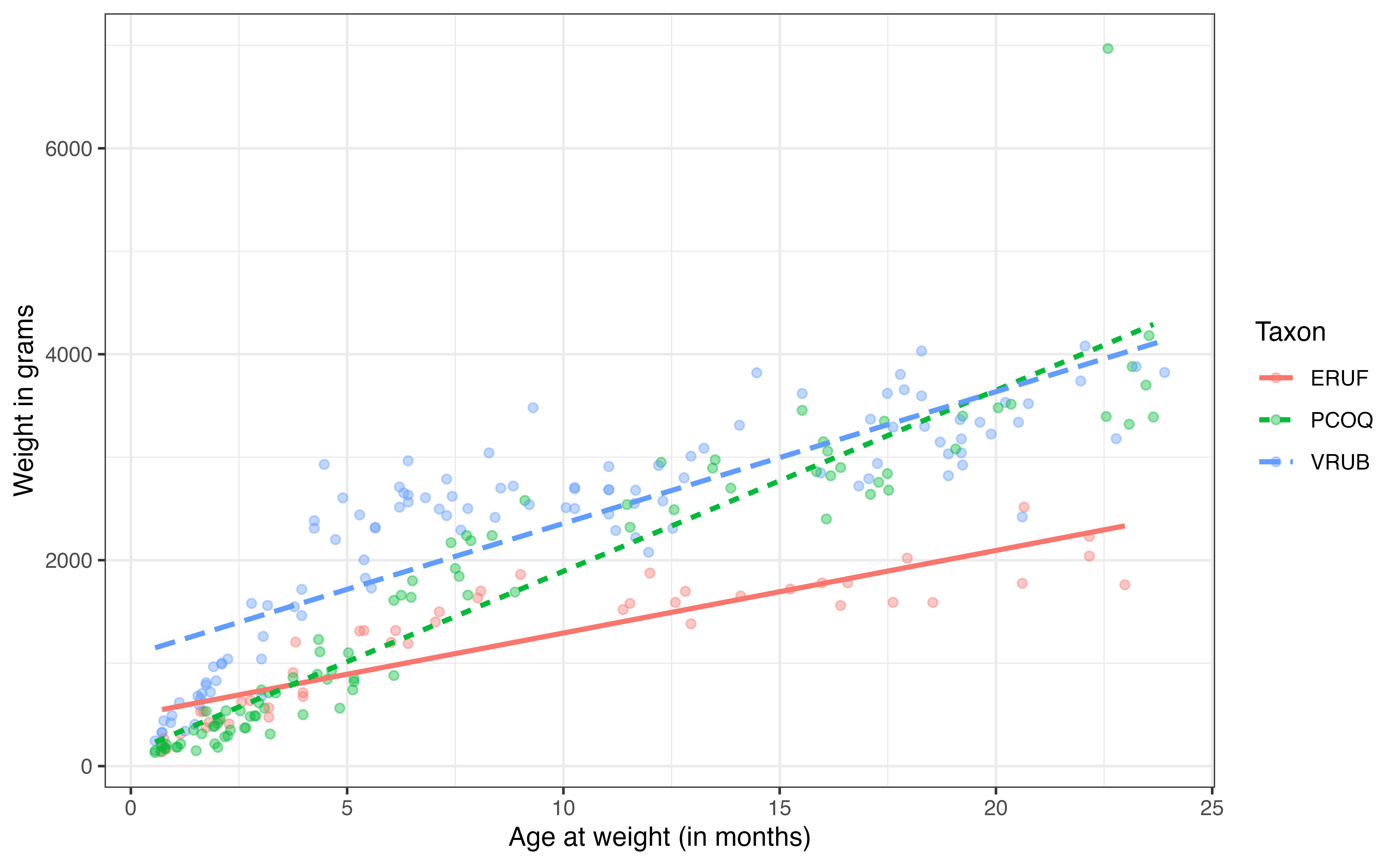
Figure 7.8: Multivariate EDA to explore potential interaction effect between age and taxon

Figure 7.8 shows the relationship between age and weight by taxon. Based on the lines, it appears that there is some difference in the relationship between age and weight depending on the taxon, as the slopes of the lines appear to differ. Thus, the plot suggests a potential interaction effect that is worth exploring in the model. If there was no potential interaction effect, then the lines would be parallel (i.e., the same slope). As with any exploratory data analysis, we do not use this plot to conclude whether or not there is an interaction effect; we will use the regression model and statistical inference for those purposes. This plot provides some intuition and guidance of what we might expect as we look at the results of the regression model.

Lemurs from which taxon appear to grow at the fastest rate?⁹

Table 7.12: Output for regression model including interaction between age and taxon

term	estimate	std.error	statistic	p.value
(Intercept)	578.8	135.43	4.274	0.000
age	78.6	9.95	7.900	0.000
sexM	-85.2	60.97	-1.398	0.163
taxonPCOQ	-355.7	134.37	-2.647	0.009
taxonVRUB	634.0	162.69	3.897	0.000
litter_size	-36.9	58.64	-0.629	0.530
age:taxonPCOQ	96.1	12.05	7.971	0.000
age:taxonVRUB	49.4	11.96	4.125	0.000

The model wit the interaction between age and taxon is in Table 7.12. The interaction terms are indicated in the output in the format var1:var2; for example, the interaction term of age for the PCOQ taxon is labeled as age:taxonPCOQ. This individual term is an estimate of how much the slope of age differs between the taxa PCOQ and ERUF, the baseline. Thus, the interpretation is

The slope of age for lemurs in the PCOQ taxon is about 96.085 greater for lemurs in PCOQ compared to lemurs in the ERUF taxon. This means for each additional month older a lemur is, the weight of a PCOQ lemur is expected to increase by 96.085 grams more, on average, compared to an ERUF lemur, holding sex and litter size constant.

This interpretation aligns with the steep slope of the line for the PCOQ species in Figure 7.8. Note from the interpretation that coefficient of the interaction effect is how much the relationship between age and weight differ for the PCOQ species compared to the ERUF species, but it is not the overall relationship between age and weight for PCOQ lemurs. To get that value, we must add the main effect of age (age) and the interaction effect (age:taxonPCOQ).

The overall slope of age for PCOQ lemurs is 174.664 (78.579 + 96.085 ). This means that among PCOQ lemurs, for each additional month in age, the weight is expected to be greater by 174.664 grams, on average, holding sex and litter size constant.

What is the slope of age for lemurs in the VRUB taxon? Interpret it in the context of the data.¹⁰

By now we have quantified the relationship between age and weight for PCOQ and VRUB lemurs, but what about this relationship for ERUF lemurs, the baseline category? The interaction effect age:taxonPCOQ is the adjustment in the slope of age for PCOQ lemurs; the same is true about age:taxonVRUB for VRUB lemurs. Therefore, neither of these interaction effects apply to ERUF lemurs. Putting all this together, the coefficient of age for ERUF lemurs is 78.579. The term in the model age is called a main effect, because it describes the relationship between the response and predictor variable (among the baseline subgroup). The terms age:taxonPCOQ and age:taxonVRUB called interaction effects, because they are how much the relationship between the response and one predictor differs by values of another predictor.

We used the original variables age and litter_size in this section; however, everything we’ve shown about interaction terms also applies to centered and standardized variables.

7.7.2 Interaction between two categorical predictors

Another type of interaction effect is between two categorical predictors. Let’s consider the interaction between taxon and sex for this data. We might include this interaction effect if we want to explore whether the relationship between sex and weight differs by taxon.¹¹

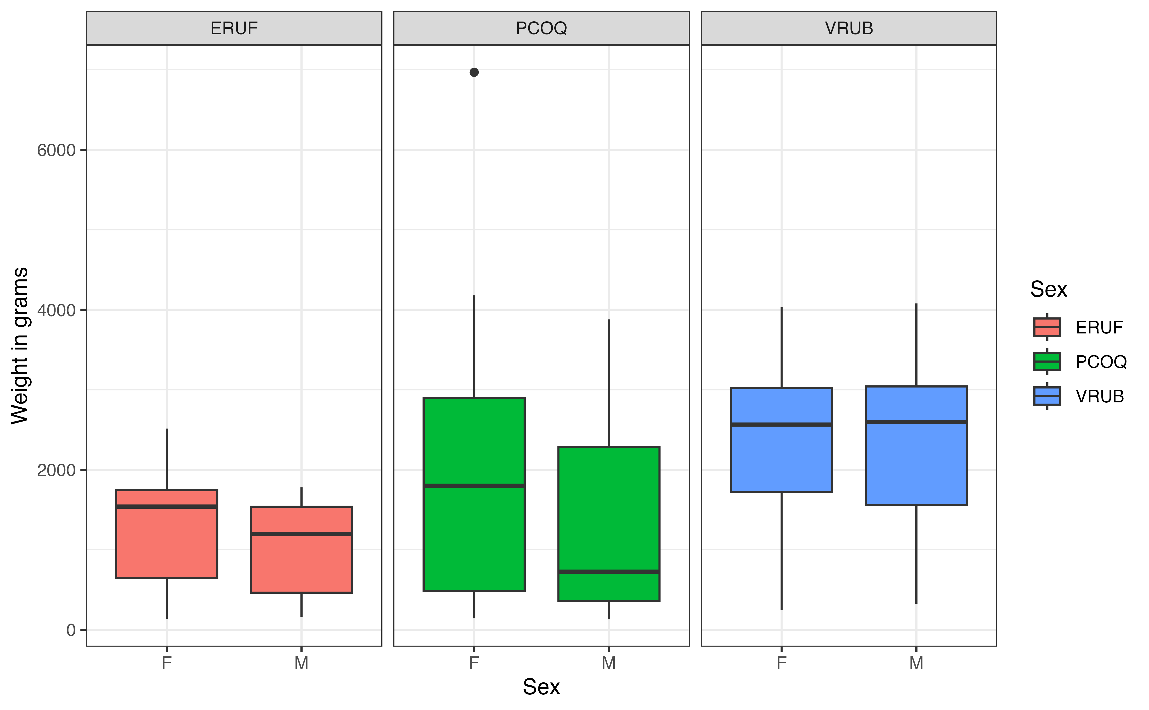
Figure 7.9: weight versus sex by taxon

Figure 7.9 shows the relationship between sex and weight by taxon. Recall that an interaction effect means that the relationship between one predictor and the response variable differs by values of another predictor. Therefore, as we examine this plot, we are looking to see whether the relationship between sex and weight appears similar or different for each taxon (see Section 3.6). When we look at the boxplots for male and female relative to one another in the figure, we don’t see much difference across the three taxa, as there is a lot of overlap between the box plots for each taxon. The median weight for males versus females appears to differ for PCOQ lemurs compared to the other two groups. Thus, from the EDA we might expect a useful interaction for sex and the PCOQ species, but maybe not for VRUB.

We add this interaction term in to the model using the same syntax as before. The output from the regression model is in Table 7.13.

Table 7.13: Output for regression model including interaction between sex and taxon

term	estimate	std.error	statistic	p.value
(Intercept)	-60.3	134.96	-0.447	0.656
age	137.1	4.88	28.102	0.000
sexM	169.2	159.26	1.063	0.289
taxonPCOQ	633.2	124.57	5.083	0.000
taxonVRUB	1124.0	152.67	7.363	0.000
litter_size	-14.4	65.58	-0.219	0.826
sexM:taxonPCOQ	-387.4	192.94	-2.008	0.046
sexM:taxonVRUB	-253.2	188.75	-1.341	0.181

Similar to the interpretations in the previous section, the interaction terms tell us how much the effect of sex among PCOQ or VRUB lemurs differ compared to the effect of sex for the baseline, ERUF lemurs. For example, the interaction term for PCOQ lemurs, sexM:taxonPCOQ = -387.382. This interpretation of this value is as follows:

The difference in the average weight of male lemurs compared to female lemurs is predicted to be 387.382 grams less for lemurs from the PCOQ taxon compared to those in the ERUF taxon, holding age and litter size constant.

As before, to get the overall difference in the average weight between male and female lemurs for the PCOQ species, we add the coefficients for the main effect sexM and the interaction effect sexM:taxonPCOQ. The overall effect of sex for PCOQ lemurs is -218.144 (169.238 + -387.382). The interpretation of this value is as follows:

For lemurs in the PCOQ taxon, the weight of male lemurs is expected to be 218.144 grams less than the weight of female lemurs, on average, holding age and litter size constant.

• What is the overall effect of sexM for lemurs in the VRUB taxon?
• What is the overall effect of sexM for lemurs in the ERUF taxon?¹²

7.7.3 Interaction between two quantitative predictors

The last type of interaction is between two quantitative predictors. This type of interaction is less common than the interactions including at least one categorical predictor, but they can be found in some scientific contexts. For the lemurs analysis, we will look at the interaction effect between age and litter_size. As with the interaction effect between two categorical predictors, we can interpret the interaction between age and litter_size as how much the effect of litter size changes as age changes or how much the effect of age changes as litter size changes. While either of these interpretations would be statistically valid, we will focus on the how the effect of litter size changes as age changes. This will allow us to more directly explore whether the impact of a lemur’s birth conditions (represented by the litter size) changes as the lemur gets older.

Visualizations for the potential interaction effect between two quantitative predictors can be complex, because a continuous predictor can take on infinitely many values. Therefore, when visualizing the potential interaction effect, we will create bins for one of the predictors and use the bins to see how the value of one of the predictors changes based on the other. Figure 7.10 is a scatterplot exploring the potential interaction between age and litter size.

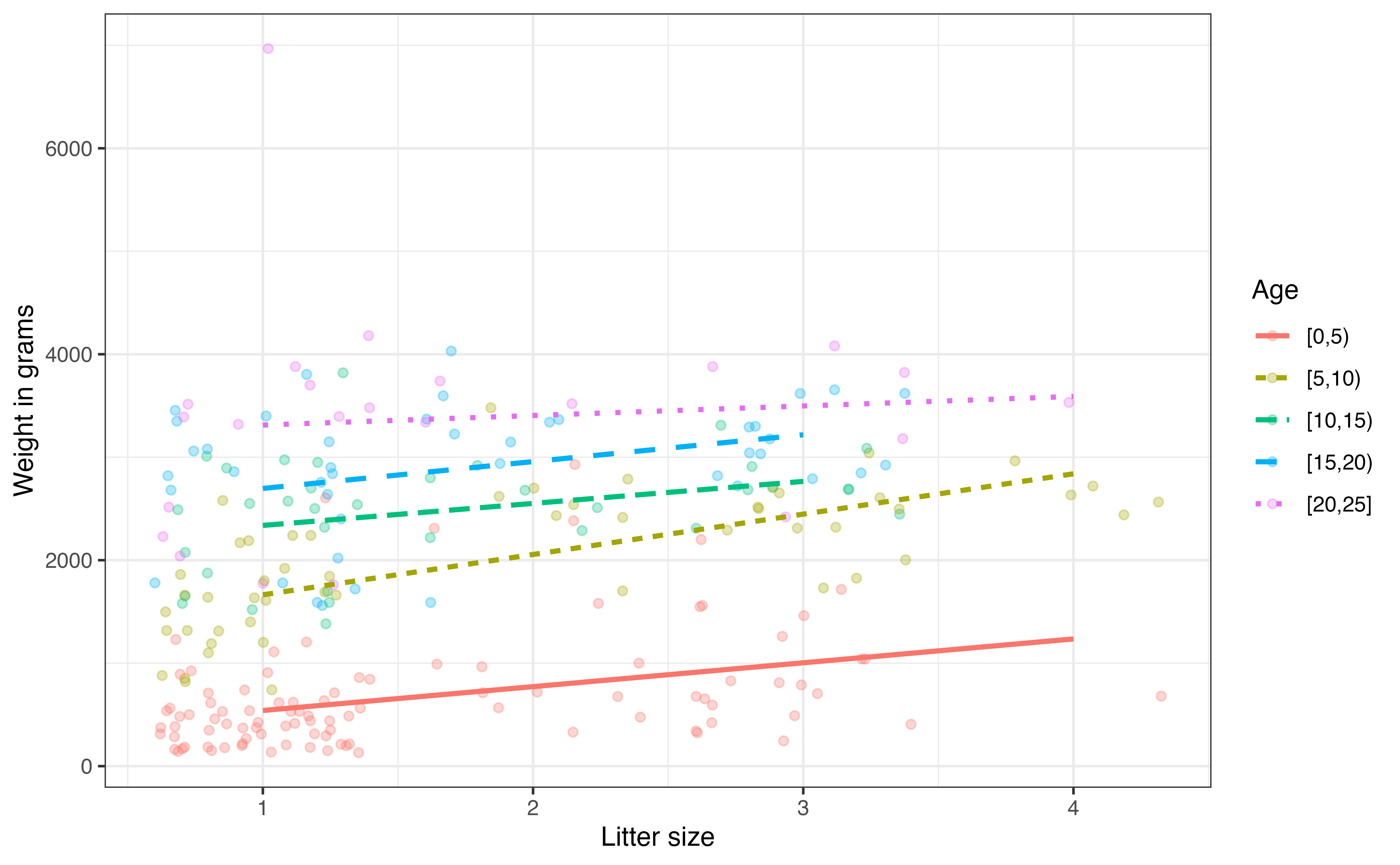
Figure 7.10: weight versus litter_size by age

Because we are specifically interested in interpreting how the effect of litter size changes as age changes, we have created bins to mark off age ranges and looked a the scatterplot of litter size and weight for each bin.

In Figure 7.10, the relationship between litter size and weight appears flatter for the older age groups, in particular the 20 - 25 month age group. This means it appears that litter size has much more impact on the weight among very young lemurs compared to those closer to two years old. As with all exploratory data analysis, we can not make a definitive conclusion based on this visualization alone, so we will fit a model with this interaction using the code below.

Table 7.14: Output for regression model including interaction between age and litter_size

term	estimate	std.error	statistic	p.value
(Intercept)	-132.3	148.49	-0.891	0.374
age	155.6	10.34	15.046	0.000
sexM	-69.6	68.22	-1.020	0.309
taxonPCOQ	477.7	94.86	5.036	0.000
taxonVRUB	1042.5	133.07	7.834	0.000
litter_size	77.4	80.78	0.958	0.339
age:litter_size	-10.9	5.33	-2.045	0.042

The output for the model with the interaction between age and litter_size is in Table 7.14. The coefficient for the term age:litter_size is the amount the effect of litter size changes as age increases by 1 month. It is interpreted as follows:

For each additional month in age, the slope of litter size and weight decreases by 10.902, on average, holding taxon and sex constant.

As with previous interaction effects, we add the coefficients for the main effect term and interaction term to get the overall effect of litter size at different ages. Recall that interaction effects are just two predictor variables multiplied together, so we need to plug in a value of age to get the overall effect of litter for that age. When we had interaction effects with at least one categorical predictor, we plugged in the 1 or 0 for the indicator variable. Now we can choose any age in the range of our data to plug in. We may also want to plug in a few different ages throughout the range to see how the effect of litter size compares for different ages.

Let’s interpret the effect of litter size for lemurs who are 12 months old. The effect of litter size for lemurs of this age is -53.4 (77.424 + 12 $\times$ -10.902). The interpretation is as follows:

For lemurs who are 12 months old, for each additional lemur in their litter, their weight is expected to be less by 53.4 grams, on average, holding sex and taxon constant.

The coefficient of the main effect of litter_size is the effect of litter size when age = 0. There are no lemurs who are 0 months old in the data, so we should be cautious about trying to derive meaning from the main effect of litter size in this model or refit the model using the centered values of the quantitative predictors.

What is the overall effect of litter size for lemurs who are 20 months old? Interpret this value in the context of the data.¹³

In this section we only discussed interactions between two variables, but there can be interactions between three or more variables. Though such interactions are possible, they should be used with caution to avoid fitting the model too closely to the sample data and losing generalizability (called model overfit). These complex interactions also become difficult to interpret and can be harder to explain to a general audience.

Therefore, we recommend only using interaction effects with two variables unless there is a specific research or analysis objective that benefits from the more complex interaction effects.

7.8 Multiple linear regression in R

7.8.1 Estimating coefficient using R

Similar to simple linear regression, we use the lm function to find the coefficient estimates ${\hat{\beta }}_0,{\hat{\beta }}_1,\dots ,{\hat{\beta }}_p$. The code to fit the the model using age, sex, taxon, and litter size to understand variability in the weight of young lemurs is shown below.

lemurs_model <- lm(weight ~ age + sex + 
                     taxon + litter_size,
                   data = lemurs)

tidy(lemurs_model) |>
  kable(digits = 3)

The tidy function structures the model output into a data data frame, and kable() is used to display the results as a neatly formatted table.

7.8.2 Prediction

We use predict() to compute predicted values from multiple linear regression models. We begin by making a tibble that contains the values fo the new observation. The variable names in the tibble of new observations must match the column names in the original data exactly, including letter case. Additionally, the observed values of the categorical predictors are put in the tibble, not indicator variables. As with variable names, the values of the categorical predictors must be input exactly as they show in the data set (including case).

new_lemur <- tibble(age = 10, 
                    taxon = "VRUB", 
                    sex = "M", 
                    litter_size = 4)
  
  
predict(lemurs_model, new_lemur)

   1 
2283 

We can also use predict() to compute the predicted values for multiple new observations. Suppose we wish to predict the weight of the following lemurs:

• Lemur 1: 10-month old male lemur in the VRUB taxon who was born into a litter of 4 lemurs (same as before)

• Lemur 2: 14-month old female lemur in the ERUF taxon who was born into a litter of 2 lemurs

We use the same process as before, extending the tibble to include the observed values for both new lemurs.

new_lemurs <- tibble(age = c(10, 14), 
                    taxon = c("VRUB", "ERUF"), 
                    sex = c("M","F"), 
                    litter_size = c(4, 2)
)
  
  
predict(lemurs_model, new_lemurs)

   1    2 
2283 1921 

Predictions using augment()

The augment function, introduced in Section 6.2, can be used to compute predicted values for each observation in the data set used to fit the model. The predicted values are stored in the column .fitted in the augmented data frame, as shown in Table 7.15.

lemurs_model_aug |>
  select(weight:.fitted) |>
  slice(1:5) |>
kable(digits = 3)

Table 7.15: Partial output from the lemurs model augumented data frame

weight	age	sex	taxon	litter_size	.fitted
410	2.27	F	ERUF	1	335
137	0.72	F	ERUF	1	123
206	0.69	F	PCOQ	1	590
185	1.05	M	PCOQ	1	551
373	2.66	F	PCOQ	1	860

7.8.3 Interaction terms

We use the asterisks * to include interaction terms between any two variables in R. The code to include the interaction between taxon and age is below.

lemurs_age_taxon_int <- lm(weight ~ age + sex + taxon + 
                             litter_size + taxon * age, 
                           data = lemurs)

tidy(lemurs_age_taxon_int)

# A tibble: 8 × 5
  term        estimate std.error statistic  p.value
  <chr>          <dbl>     <dbl>     <dbl>    <dbl>
1 (Intercept)    579.     135.       4.27  2.76e- 5
2 age             78.6      9.95     7.90  9.51e-14
3 sexM           -85.2     61.0     -1.40  1.63e- 1
4 taxonPCOQ     -356.     134.      -2.65  8.65e- 3
5 taxonVRUB      634.     163.       3.90  1.26e- 4
6 litter_size    -36.9     58.6     -0.629 5.30e- 1
# ℹ 2 more rows

The syntax to include the interaction between two quantitative variables is the same as the other interactions. Note also that even though we used the binned values of age to help visualize the potential interaction effect in Figure 7.10, we use the original non-binned values of age in the model.

lemurs_age_litter_int <- lm(weight ~ age + sex + taxon + 
                             litter_size + age * litter_size, 
                           data = lemurs)

7.9 Summary

In this chapter, we introduced multiple linear regression, in which two or more predictor variables are used to understand variability and compute predictions for a quantitative response variable. We introduced a various different predictors that can be in the model, including categorical predictors and interaction terms. We showed how to use R to estimate model coefficients and compute predictions from the model. We expect there is uncertainty in the coefficient estimates produced by the regression model, given it was fit using sample data. In the next chapter, we will discuss inference for multiple linear regression and use it to draw conclusions about the relationships between the response and predictor variables.

Community, Data Science Learning. 2024. “Tidy Tuesday: A Weekly Social Data Project.” https://tidytues.day.

Duke Lemur Center. n.d. “Meet the Lemurs.” https://lemur.duke.edu/discover/meet-the-lemurs/.

James, Gareth, Daniela Witten, Trevor Hastie, and Robert Tibshirani. 2021. An Introduction to Statistical Learning: With Applications in r. 2nd ed. Springer.

Zehr, SM, RG Roach, D Haring, J Taylor, FH Cameron, and AD Yoder. n.d. “Life History Profiles for 27 Strepsirrhine Primate Taxa Generated Using Captive Data from the Duke Lemur Center. Sci Data. 2014; 1: 140019.”

---

1. The distribution of age is unimodal and skewed right, so the center is best described by the median 7.1 months and spread by the IQR of 12.8 months. There does not appear to be any outliers for age in the data.

2. It is possible to fit models such that $p>n$. These models are beyond the scope of this text, so we refer the reader to Chapter 6 of James et al. (2021) for further reading.

3. For each additional lemur in the litter in which a young lemur was born, the weight is expected to be lower by 19.607 grams, holding taxon, sex, and age constant.

4. The baseline level for sex is “F” (Female). The average weight for male lemurs is about 88.838 grams less than the average weight for female lemurs, holding taxon, age, and litter size constant. The intercept for female lemurs is 43.844 .The intercept for male lemurs is -44.994 (43.844 + -88.838 ).

5. It is not, because it is not possible for a lemur to be born into a litter of size 0. The litter size must be at least 1.

6. $\widehat{\text{weight\_g}}=43.844+136.903\times 14-88.838\times 0+471.715\times 0+1037.323\times 0-19.607\times 2=1921.272$$

7. We only centered or standardized the quantitative predictors; we have not changed the categorical predictors. Recall that the indicator variables shift the intercept, and thus this did not change though the relationship between the response and the quantitative predictors may have changed.

8. The variable litter_size , because it has the coefficient with the smallest magnitude, |18.128 |= 18.128 .

9. Lemurs in the PCOQ taxon appear to grow at the fastest rate, because its line in Figure 7.8 (green dotted line) is the steepest.

10. The slope of age for lemurs in the VRUB taxon is 127.931 (78.579 + 49.352). This means that among VRUB lemurs, for each additional month in age, the weight is expected to be greater by 127.931 grams, on average, holding sex and litter size constant.

11. The interaction between sex and taxon would also tell us if the relationship between taxon and weight differs by sex. We have decided to interpret the interaction effect in the other direction given it is more practically meaningful to understand differences between sexes within each taxon versus the other way around.

12. The overall effect of sexM for lemurs in the VRUB taxon is -83.971 (169.238 + -253.209 ). The overall effect of sexM for lemurs in the ERUF taxon is 169.238

13. The overall effect of litter size for lemurs who are 20 months old is 66.522 . This means that for lemurs who are 20 months old, for each additional sibling in their litter, their weight is expected to be less by 140.616 (77.424 + 20 $\times$ -10.902 ), on average, holding sex and taxon constant.