12  Logistic regression: Prediction and evaluation

Learning goals

• Compute predictions from the logistic regression model
• Use model predictions to classify observations
• Construct and interpret a confusion matrix
• Use the ROC curve to evaluate model performance and select classification threshold
• Evaluate model performance using AUC, AIC, and BIC
• Implement a model building workflow for logistic regression using R

12.1 Introduction: Predicting comfort with driverless cars

In Chapter 11, we introduced data from the 2024 General Social Survey in which adults in the United States their opinions were asked on a variety of issues, including their comfort with driverless cars. In the previous chapter, we fit a logistic regression model used the model to describe the characteristics associated with the odds an adult is comfortable with driverless cars. We continue with the analysis in this chapter, with a focus on using the model for prediction. We will also evaluate the model performance and show an example workflow for comparing two logistic regression models.

We use the variables below in this chapter. The variable definitions are based on survey prompts and variable definitions in the General Social Survey Documentation and Public Use File Codebook (Davern et al. 2025).

• aidrive_comfort: Indicator variable for respondent’s comfort with driverless (self-driving) cars. 0: Not comfortable at all; 1: At least some comfort.

  • This variable was derived from responses to the original survey prompt: “Comfort with driverless cars”. Scores ranged from 0 to 10 with 0 representing “totally uncomfortable with this situation” and 10 representing “totally comfortable with this situation”. Responses of 0 on the original survey were coded as aidrive_comfort = 0. All other responses coded as 1.

• tech_easy : Response to the question, “Does technology make our lives easier?” Categories are Neutral, Can't choose (Respondent doesn’t know / is unable to provide an answer), Agree, Disagree.

• age: Respondent’s age in years

• income: Response to the question “In which of these groups did your total family income, from all sources, fall last year? That is, before taxes.” Categories are Less than $20k, $20-50k, $50-110k, $110k or more, Not reported .

  • Note: These categories were defined based on the 27 categories in income16 from the original survey.

• tech_harm: Response to the question, “Does technology do more harm than good?”. Categories are Neutral, Can't choose (Respondent doesn’t know / is unable to provide an answer), Agree, Disagree.

• polviews: Response to the question, “I’m going to show you a seven-point scale on which the political views that people might hold are arranged from extremely liberal–point 1–to extremely conservative–point 7. Where would you place yourself?” Categories are Moderate, Liberal, Conservative, No reported.

  • Note: These categories were defined based on the original 7 point scale.

12.2 Exploratory data analysis

12.2.1 Univariate EDA

We conducted exploratory data analysis for the response variable aidrive_comfort and the predictors age and tech_easy in Section 11.1. Here we focus on EDA for the new predictors and their relationship with the response variable.

(a) income

(b) polviews

(c) tech_harm

Figure 12.1: Univariate exploratory data analysis

Figure 12.1 shows the distributions of the predictors that are new in this chapter. From the distribution of income in Figure 12.1 (a) , we see that the most common response for income is between $50-110K. There is a sizable proportion of the respondents who did not report an income. Studies have shown that failure to report income in surveys is not random (e.g., Jabkowski and Piekut 2024), so it will be worth noting if the Not Reported indicator has a statistically significant relationship with the response variable as we continue the analysis.

The distribution of polviews_fct in Figure 12.1 (b) shows a relatively even distribution along the range of political views. A few respondents chose not to report their political views. Lastly, the distribution of tech_harm in Figure 12.1 (c) shows that most people either disagree are have neutral feelings about the statement that technology causes more harm than good.

12.2.2 Bivariate EDA

(a) aidrive_comfort vs. income

(b) aidrive_comfort vs. polviews

(c) aidrive_comfort vs. tech_harm

Figure 12.2: Bivariate exploratory data analysis. Blue: adrive_comfort = 0, Red: aidrive_comfort = 1

The visualizations in Figure 12.2 show the relationships between the response variable and each new predictor variable. Figure 12.2 (a) shows the relationship between income and aidrive_comfort. The graph shows that a higher proportion of respondents in the higher income categories are comfortable with driverless cars compared to respondents in lower income categories or who did not report income. This suggests an individual’s income may be useful in understanding the chance they are comfortable with driverless cars.

The relationship between polviews and aidrive_comfort is in Figure 12.2 (b). Those who identify as “liberal” on the political spectrum are the most likely to be comfortable with driverless cars, and those who did not report a political affiliation are the least likely. Those who identify as “moderate” or “conservative” have about the same odds of being comfortable with driverless cars.

Lastly, Figure 12.2 (c) is the relationship between tech_harm and aidrive_comfort. Those who disagree that technology causes more harm than good are the most likely to be comfortable with driverless cars. Those who did not provide a response or agree that technology causes more harm than good are the least likely to be comfortable with driverless cars.

12.2.3 Initial model

We begin by fitting a model using the predictors from Chapter 11, age and tech_easy, along with a new predictor income to predict whether an individual is comfortable with driverless cars. We’ll use this model for the majority of the chapter as we introduce prediction, classification, and model assessment for logistic regression. In Section 12.7, we’ll use cross validation and the model selection workflow from Chapter 10 to compare this model to another one that also includes polviews and tech_harm.

Table 12.1: Model of aidrive_comfort versus age, tech_easy, and income with 95% confidence intervals

term	estimate	std.error	statistic	p.value	conf.low	conf.high
(Intercept)	0.032	0.237	0.136	0.892	-0.433	0.496
age	-0.016	0.003	-5.165	0.000	-0.022	-0.010
tech_easyCan’t choose	0.075	0.408	0.184	0.854	-0.746	0.866
tech_easyAgree	0.576	0.155	3.730	0.000	0.275	0.881
tech_easyDisagree	-0.436	0.300	-1.456	0.145	-1.039	0.140
income_fct$20-50k	0.264	0.177	1.491	0.136	-0.082	0.612
income_fct$50-110k	0.526	0.169	3.111	0.002	0.196	0.860
income_fct$110k or more	1.223	0.182	6.704	0.000	0.868	1.584
income_fctNot reported	0.265	0.219	1.212	0.225	-0.164	0.694

Consider the coefficients for the indicators of income_fct. Are they consistent with the observations from the EDA? Why or why not. ¹

12.3 Prediction and classification

In Chapter 11, we introduced the logistic regression, where we used the model to describe and draw conclusions about the relationship between the response and predictor variables. In practice, logistic regression models are widely used for classification, particularly in data science and machine learning. They are part of a branch of machine learning models called supervised learning, in which the model is built and evaluated using data that contains observed outcomes. Therefore, we will now focus on using the model to predict whether an individual is comfortable with self-driving cars given particular characteristics.

12.3.1 Prediction

Recall from Section 11.3 that the response variable in the logistic regression model is the logit (log-odds). When we input values of age, tech_easy, and income into the model in Table 12.1, the model will output the log odds an individual with those characteristics is comfortable with driverless cars. Once we have the predicted log odds, we can use the relationships in Section 11.2 to compute the predicted odds and the predicted probability. Table 12.2 shows the predicted log odds, predicted odds, and predicted probability for 10 observations in the data set.

Table 12.2: Predictions from model in Table 12.1 for 10 respondents

	aidrive_comfort	age	tech_easy	income	Pred. log odds	Pred. odds	Pred. probability
1	1	33	Agree	$110k or more	1.306	3.692	0.787
2	1	19	Neutral	$110k or more	0.953	2.593	0.722
3	0	25	Can’t choose	Not reported	-0.026	0.974	0.494
4	0	68	Neutral	Less than $20k	-1.052	0.349	0.259
5	0	63	Can’t choose	Less than $20k	-0.897	0.408	0.290
6	0	31	Agree	$50-110k	0.641	1.899	0.655
7	0	63	Agree	$110k or more	0.828	2.288	0.696
8	1	41	Agree	$50-110k	0.482	1.619	0.618
9	1	75	Agree	$20-50k	-0.323	0.724	0.420
10	1	51	Agree	$110k or more	1.019	2.771	0.735

Let’s show how the predicted values for the first observation are computed. The predicted log odds the first individual who is 33 years old, agrees that technology makes life better, and has an annual income of $110k or more are

\[ \begin{aligned} \log \Big(\frac{\hat{\pi}}{1-\hat{\pi}}\Big) &= 0.032 - 0.016 \times 33 + 0.075 \times 0 + 0.576 \times 1 \\ &- 0.436 \times 0 + 0.264 \times 0 + 0.526 \times 0 \\ & + 1.223 \times 1 + 0.265 \times 0 \\ & = 1.3 \end{aligned} \]

where \(\hat{\pi}\) is the predicted probability of being comfortable with driverless cars.

Using the predicted log odds from Table 12.2, the predicted odds for this individual are

\[\widehat{\text{odds}} = e^{\log \big( \frac{\hat{\pi}}{1-\hat{\pi}}\big)} = e^{1.306} = 3.69 \]

Lastly, we use the odds from Table 12.2 to compute the predicted probability:

\[ \hat{\pi} = \frac{\widehat{\text{odds}}}{1 + \widehat{\text{odds}}} = \frac{3.692}{1 + 3.692} = 0.787 \]

Note: These values may differ slightly from the values in the the table, because we are computing predictions using rounded coefficient.

Show how to compute the predicted log odds, odds, and probability for individual #2 in Table 12.2.²

12.3.2 Classification

Knowing the predicted odds and probabilities can be useful for understanding how likely individuals with various characteristics will be comfortable with driverless cars. In many contexts, however, we would like to group individuals based on whether or not the model predicts they are comfortable with driverless cars. For example, the marketing team for a robotaxi company may want to use targeted marketing strategies and offer discounts to potential new customers. To have a successful marketing campaign, they want to direct the marketing to those who are comfortable with driverless cars.

As we’ve seen thus far, the logistic regression model does not directly produce predicted values of the binary response variable. Therefore, we can group observations based on the predicted probabilities computed from the model output. This process of grouping observations based on the predictions is called classification. The groups the observations are put into are the predicted classes. In the case of our analysis, we will use the model to classify observations into the class of those not comfortable with driverless cars (aidrive_comfort = 0) or the class of those comfortable with driverless cars (aidrive_comfort = 1) .

We showed how to compute the predicted probabilities from the logistic regression output in Section 12.3.1, and we will use those probabilities to classify observations. The question, then, is how large does the probability need to be to classify an observation as having the response \(Y = 1\) ? In terms of our analysis, how large does the probability of being comfortable with driverless cars need to be to classify an individual as being comfortable with driverless cars, aidrive_comfort = 1?

When using the logistic regression model for classification, we define a threshold, such an observation is classified as \(\hat{Y} = 1\) if the predicted probability is greater than the threshold. Otherwise, the observation is classified as \(\hat{Y} = 0\). If we’re unsure what threshold to set, we can start with a threshold of 0.5, the default threshold typically used in statistical software. This means if the model predicts an observation is more likely than not to have response \(Y = 1\), even if just by a small amount, then the observation is classified as having response \(\hat{Y} = 1\).

For now, let’s use the threshold equal to 0.5 to assign the predicted classes of aidrive_comfort for the respondents in the sample data based on the predicted probabilities produced from the model in Table 12.1.

Table 12.3: Predicted class based on model in Table 12.1 and threshold of 0.5 for 10 respondents

	aidrive_comfort	Pred. probability	Pred. class
1	1	0.787	1
2	1	0.722	1
3	0	0.494	0
4	0	0.259	0
5	0	0.290	0
6	0	0.655	1
7	0	0.696	1
8	1	0.618	1
9	1	0.420	0
10	1	0.735	1

Table 12.3 shows the observed value of the response (aidrive_comfort), predicted probability, and predicted class for ten respondents. For many of these respondents, the observed and predicted classes are equal. There are some, such as Observation 6, in which the predicted classes differs from the observed. In this instance, the respondent had a combination of age, income, and tech_easy, that are associated with a higher probability of being comfortable with driverless cars; however, the individual responded they are not comfortable with driverless cars in the General Social Survey.

We need a way to more holistically evaluate how well the predicted classes align with the observed classes. To do so, we use a confusion matrix, a \(2 \times 2\) table of the observed classes versus the predicted classes.

Table 12.4: Confusion matrix for model in Table 12.1 and threshold of 0.5. Observed class (columns), Predicted class (rows)

	Observed class
Pred. class	0	1
0	349	228
1	343	601

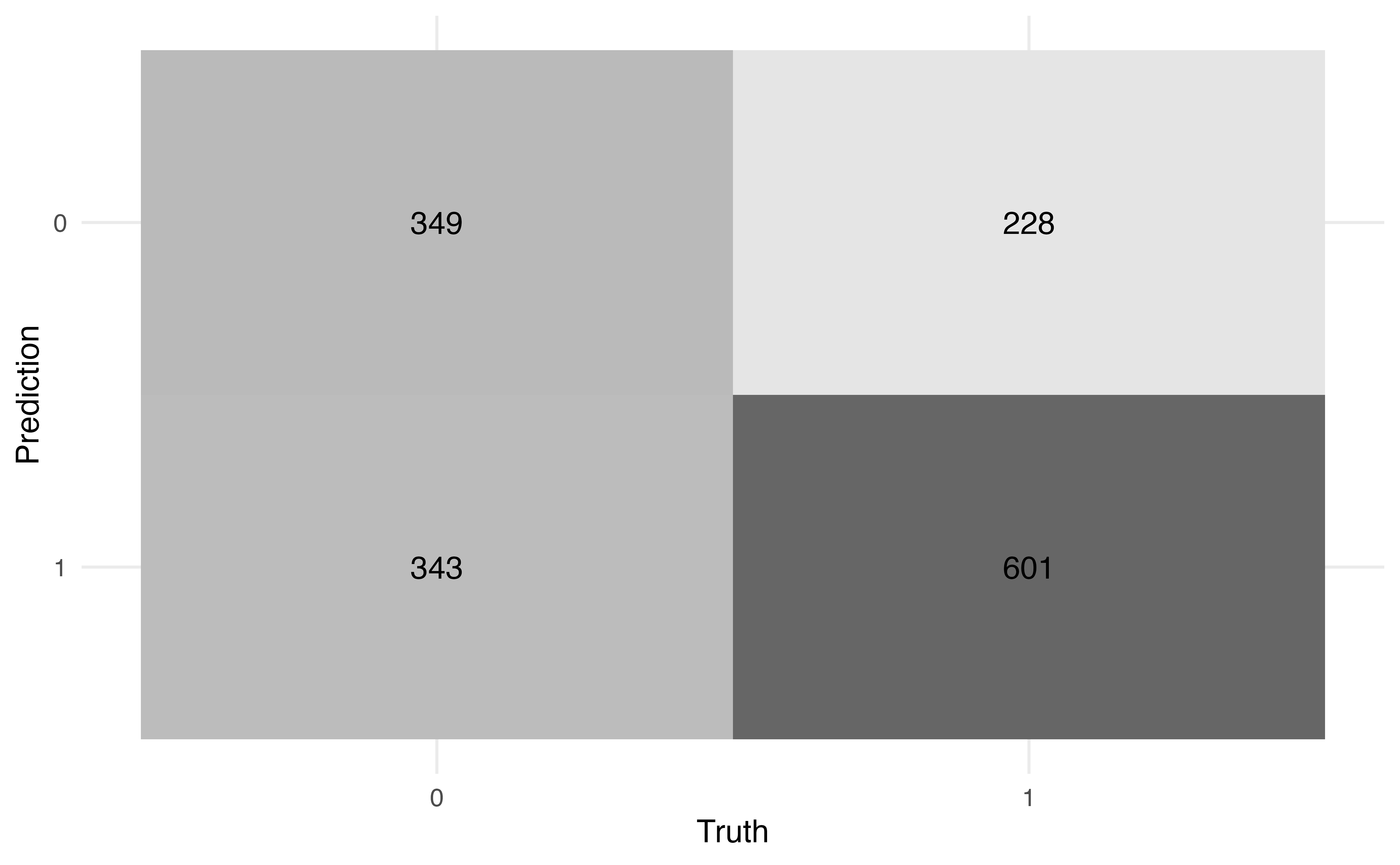
Table 12.4 shows the confusion matrix for the model in Table 12.1 and a threshold of 0.5. In this table, the rows define the predicted classes and the columns define the observed classes. Let’s break down what each cell is in the table:

• There are 349 observations with the predicted class of 0 and observed class of 0.
• There are 228 observations with the predicted class of 0 and observed class of 1.
• There are 343 observations with the predicted class of 1 and observed class of 0.
• There are 601 observations with the predicted class of 1 and observed class of 1.

We compute various statistics from the confusion matrix to evaluate how well the observations are classified. The first statistics we can calculate are the accuracy and misclassification rate. The accuracy is the proportion of observations that are correctly classified (the observed and predicted classes are the same). The accuracy based on Table 12.4 is

\[ \text{accuracy} = \frac{349 + 601}{349 + 228 + 343 + 601} = 0.625 \tag{12.1}\]

Using the model in Table 12.1 and the threshold of 0.5, 62.5% of the observations are correctly classified.

The misclassification rate is the proportion of observations that are not correctly classified (the observed and predicted classes differ). The misclassification rate based on Table 12.4 is

\[ \text{misclassification} = \frac{228 + 343}{349 + 228 + 343 + 601} = 0.375 \tag{12.2}\]

Using the model in Table 12.1 and the threshold of 0.5, 37.5% of the observations are incorrectly classified. Note that the misclassification rate is equal to \(1 - \text{accuracy}\) ,and vice versa.

When the distribution of the response variable is largely imbalanced, the accuracy can be a misleading measure of how well the observations are classified. For example, suppose there are 100 observations, such that 5% of the observations have an observed response \(Y = 1\), and 95% of the observations have an observed response of \(Y = 0\). We may observe an imbalanced distribution like this when building a model to detect the presence of a rare disease, for example.

Let’s suppose based on the model and threshold, all observations have a predicted class of 0, and the confusion matrix looks like the following:

	Observed class
Pred. class	0	1
0	95	5
1	0	0

The accuracy for this model will be (95 + 0 ) / (95 + 5) = 0.95. Based on this value, it appears the classification has performed very well, even though we did not accurately classify any of the observations in which the observed response is \(Y = 1\).

The accuracy and misclassification rate provide a nice initial indication of the how well the model classifies observations, but they do not give a complete picture. For example, suppose we want to know how many of the people who are actually comfortable with driverless cars are predicted to be comfortable based on the model predictions and threshold. Or suppose we want to know how many people who are actually not comfortable with driverless cars were incorrectly classified as being comfortable. To answer these and similar questions, let’s take a more detailed look at the confusion matrix.

Table 12.5: Detailed confusion matrix

	Not comfortable with driverless cars \((y_i = 0)\)	Comfortable with driverless cars \((y_i = 1)\)
Classified not comfortable\((\hat{y}_i = 0)\)	True negative (TN)	False negative (FN)
Classified comfortable\((\hat{y}_i = 1)\)	False positive (FP)	True positive (TP)

Table 12.5 shows in greater detail what is being quantified in each cell of the confusion matrix. We will use these values to compute more granular values about the classification. As in Table 12.4, the rows define the predicted classes and the columns define the observed classes. The values in the cell indicate the following:

• True negative (TN): The number of observations that are predicted to be not comfortable with driverless cars ( \(\hat{y}_i = 0\)) and have observed response of not comfortable (\(y_i = 0\)) .

• False negative (FN): The number of observations that are predicted to be not comfortable with driverless cars ( \(\hat{y}_i = 0\)) and have observed response of comfortable ( \(y_i = 1\)) .

• False positive (FP): The number of observations that are predicted to be comfortable with driverless cars ( \(\hat{y}_i = 1\)) and have observed response of not comfortable ( \(y_i = 0\)) .

• True positive (TP): The number of observations that are predicted to be comfortable with driverless cars ( \(\hat{y}_i = 1\)) and have observed response of comfortable ( \(y_i = 1\)) .

Using these definitions, the general form of accuracy computed in Equation 12.1 is

\[ \text{accuracy} = \frac{\text{True negative} + \text{True positive}}{\text{True negative} + \text{False negative} + \text{False positive} + \text{True positive}} \tag{12.3}\]

Write the general equation for the misclassification computed in Equation 12.2 using the terms in Table 12.5.³

Now let’s take a look at additional statistics that help us quantify how well the observations are classified. First, we’ll focus on the column containing those who have observed values \(y_i = 1\).

The sensitivity (true positive rate) is the proportion of those with observed \(y_i = 1\) that were correctly classified as \(\hat{y}_i = 1\). In machine learning contexts, this value is also called recall or probability of detection.

\[ \text{Sensitivity} = \frac{\text{True positive}}{\text{False negative} + \text{True positive}} \tag{12.4}\]

The false negative rate is the proportion of those with observed \(y_i = 1\) that were incorrectly classified as \(\hat{y}_i = 0\).

\[ \text{False negative rate} = \frac{\text{False negative}}{\text{False negative} + \text{True positive}} \tag{12.5}\]

The false negative rate is equal to \(1 - \text{Sensitivity}\) and vice versa. The denominators for the false negative rate and the sensitivity are the total number of observations with observed response \(y_i = 1\). In terms of our analysis, this is the total number of people who responded they are comfortable with driverless cars in the General Social Survey.

Next, we look at the column of containing those who have observed values of \(y_i =0\).

The specificity (true negative rate) is the proportion of those with observed \(y_i = 0\) who were correctly classified as \(\hat{y}_i = 0\).

\[ \text{Specificity} = \frac{\text{True negative}}{\text{True negative} + \text{False positive}} \tag{12.6}\]

The false positive rate is the proportion of those with observed \(y_i = 0\) who were incorrectly classified as \(\hat{y}_i = 1\). In machine learning contexts, this value is also called the probability of false alarm.

\[ \text{False positive rate} = \frac{\text{False positive}}{\text{True negative} + \text{False positive}} \tag{12.7}\]

The false positive rate is equal to \(1 - \text{specificity}\). The denominators for the specificity and false positive rate are the total number of observations with observed response \(y_i = 0\). In terms of our analysis, this is the total number of people who responded they are not comfortable with driverless cars in the General Social Survey.

The values shown thus far quantify how well observations are classified based on the observed response. Another question that is often of interest is among those with predicted class of \(\hat{y}_i = 1\), how many actually have observed values of \(y_i = 1\)? This value is called the precision.

\[ \text{Precision} = \frac{\text{True positive}}{\text{False positive} + \text{True positive}} \tag{12.8}\]

Now the denominator is the number of observations that have a predicted class \(\hat{y}_i = 1\), the second row in the Table 12.5. In the context of our analysis, the precision is how many of the individuals who are predicted to be comfortable with driverless cars actually responded on the General Social Survey that they are comfortable with driverless cars. If we’re using the model to identify individuals for a targeted marketing campaign, the precision can be useful in quantifying whether the marketing will generally capture those who are actually comfortable with driverless cars or if a large proportion would be aimed at those who actually aren’t comfortable with driverless cars and likely won’t become robotaxi customers.

Use Table 12.4 to compute the following:

• Sensitivity

• Specificity

• Precision⁴

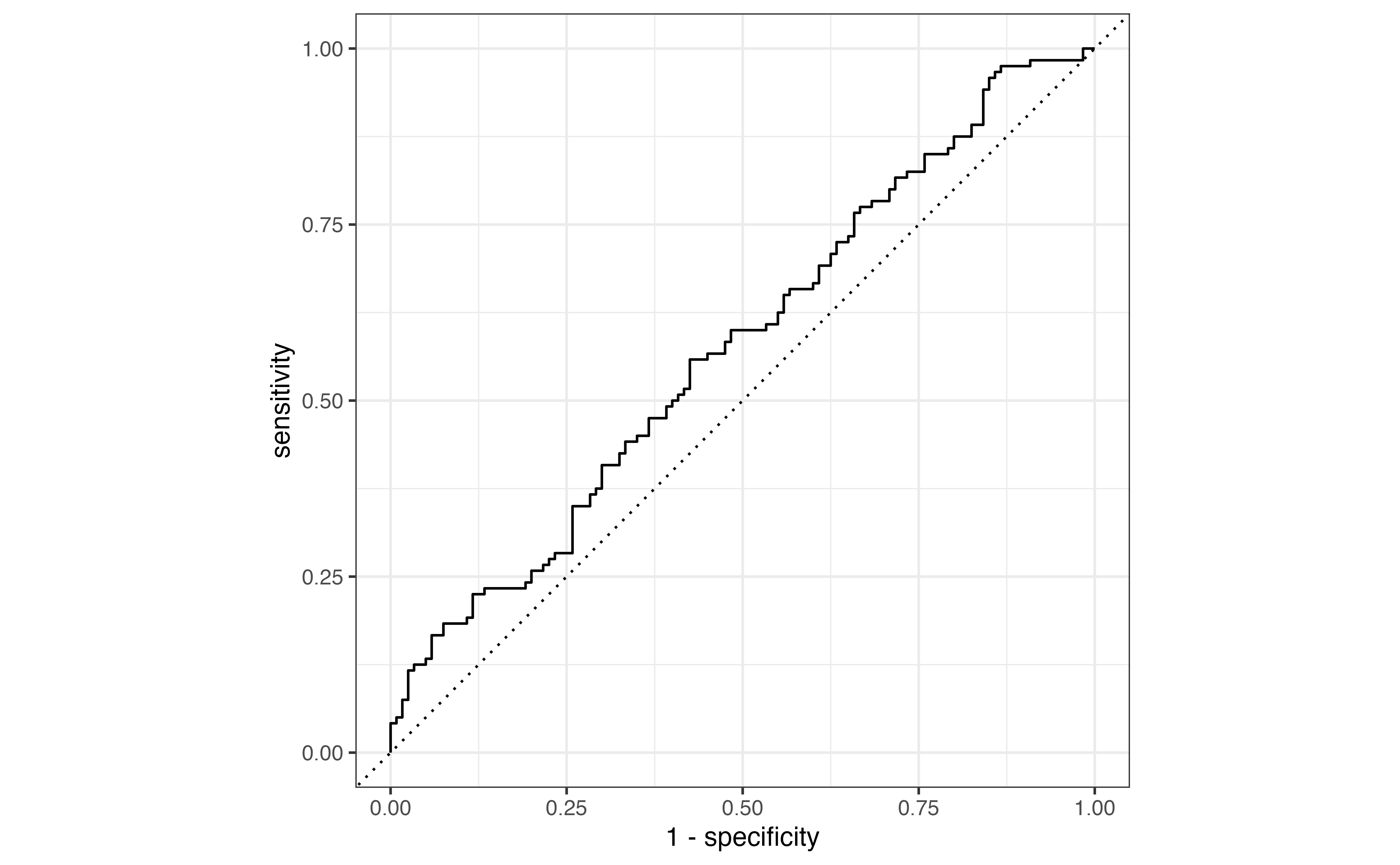
We have shown how we can derive a lot of useful information from the confusion matrix. As we use the confusion matrix to evaluate how well observations are classified; however, we need to keep in mind that the confusion matrix is determined based on the model predictions and the threshold for classification. For example, in Table 12.6, we see a confusion matrix for the same model in (aidrive-comfort-fit?) using the threshold of 0.3.

Table 12.6: Confusion matrix using model in Table 12.1 and threshold of 0.3

	Observed class
Pred. class	0	1
0	70	15
1	622	814

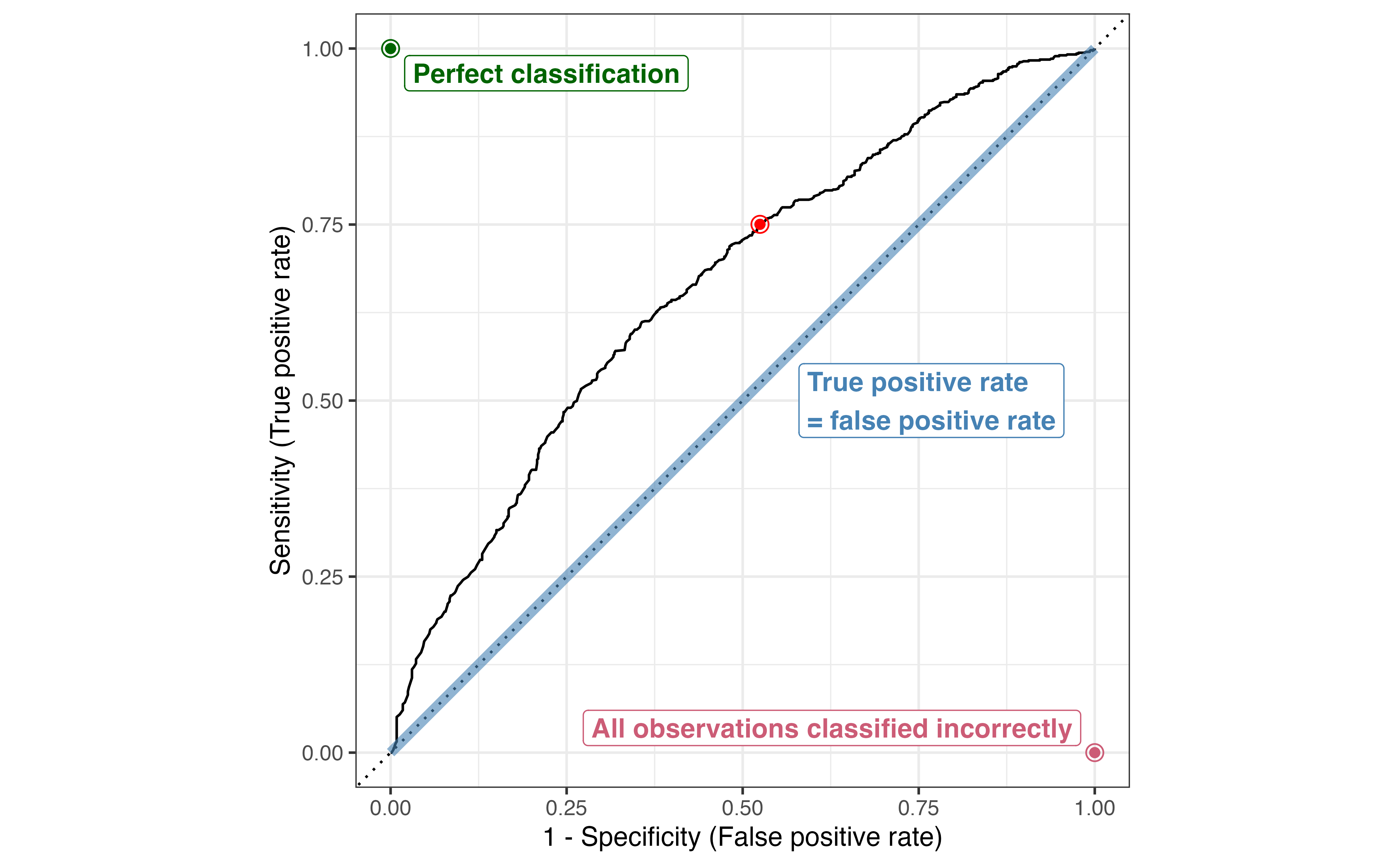
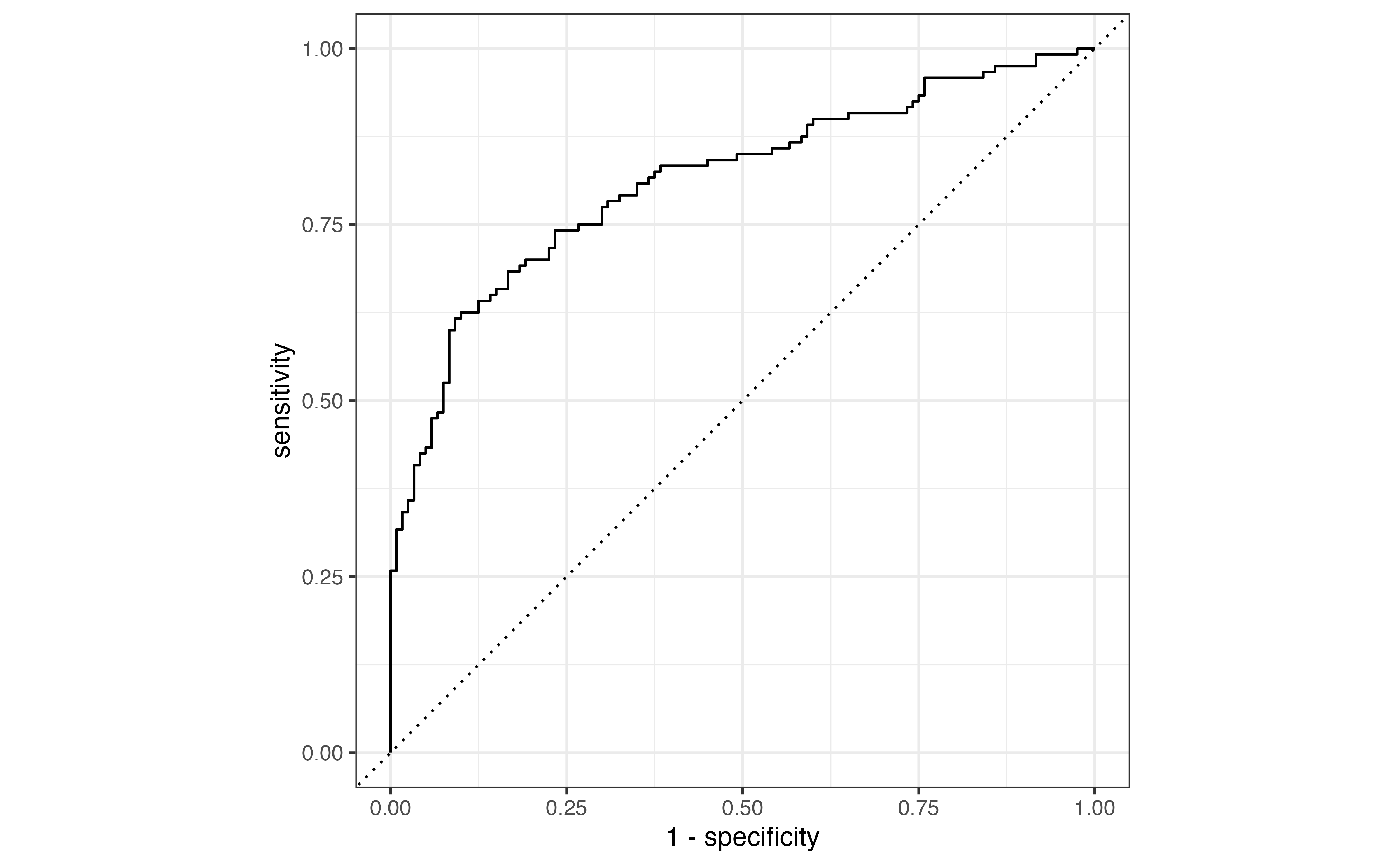
Due to the low threshold, there are many more observations classified as \(\hat{y}_i = 1\) compared to Table 12.4. The accuracy rate is now 58.1% and the misclassification rate is 41.9% even though the model hasn’t changed. From this example, we see that even if the model is unchanged, the metrics computed from the confusion matrix will differ based on the threshold. Therefore, we would like a way to evaluate the model performance independent from the choice of threshold.

12.4 ROC Curve

Ideally, we want a way to evaluate the the model performance regardless of threshold and then choose a threshold that results in the “best” classification as determined by the statistics from the previous section. We could make confusion matrices across a range of thresholds, but this process could be cumbersome and time consuming to make so many confusion matrices. Rather than make individual confusion matrices, we will use the receiving operator characteristic (ROC) curve shown in Figure 12.3. The ROC curve is a single visualization to holistically evaluate the model fit and see how well the model classifies at different thresholds. We can use the data from the ROC curve to choose a classification threshold.

Figure 12.3: ROC curve for model in Table 12.1 with point marked at threshold = 0.4754

Figure 12.3 is the ROC curve for the model in Table 12.1. The \(x\)-axis on the ROC curve is \(1 - \text{Specificity}\), the false positive rate, and the \(y\)-axis is \(\text{Sensitivity}\), the true positive rate. Thus, the ROC curve is a visualization of the true positive rate versus the false positive rate at classification thresholds ranging from 0 to 1 (equivalent to the log odds ranging from \(-\infty\) to \(\infty\)). The diagonal line represents a model fit in which the true positive rate and false positives are equal regardless of the threshold. This means the model is unable to distinguish the observations that actually have an observed response of \(y_i = 1\) versus those that do not, so it is essentially the same as using a coin flip to classify observations (not a good model!). In contrast, ROC curves that hit closer to the top-left corner indicate a model that is good at distinguishing true positives and false positives.

(a) Poor distinction

(b) Good distinction

(c) Nearly perfect distinction

Figure 12.4: Example ROC curves for different model performs

Figure 12.4 shows example ROC curves for different model fits. Figure 12.4 (a) is the ROC curve for a model that does a poor job distinguishing between the true positives and false positives (close to the diagonal line) and Figure 12.4 (c) is the ROC curve for a model that almost perfectly distinguishes between the true and false positives (close to the top-left corner). Generally, we expect to see ROC curves somewhere in the middle, similar to Figure 12.4 (b). Here, the model generally does a good job distinguishing between the true and false positives, but we will expect to get some false positives if we want a high true positive rate (sensitivity).

Each point in the ROC curve is \((1 - \text{Specificity, } \text{Sensitivity})\) at a given threshold and can be thought of as representing an individual confusion matrix for a given threshold. For example, the point marked in red on the ROC curve in Figure 12.3 shows corresponds to \(1 - \text{Specificity} = 0.525\) and \(\text{Sensitivity} = 0.75\). This point corresponds to the classification threshold 0.4888088. The corresponding confusion matrix is shown in Table 12.7. Observations with predicted probability \(\hat{\pi}_i > 0.4888088\) are classified as being comfortable with driverless cars, and those with \(\hat{\pi}_i \leq 0.4888088\) are classified as not being comfortable with driverless cars.

Table 12.7

	Observed class
pred_class3	0	1
0	329	207
1	363	622

Compute the sensitivity and specificity from Table 12.7 and compare these to the values observed on the curve in ?fig-aidrive-roc.

In the next section, we will talk more about using the ROC curve to evaluate the model fit beyond a visual assessment. For now, let’s discuss how to use the ROC curve to determine a probability threshold for classification. When we use a model for classification, we want a high true positive rate and a low false positive rate. Therefore, one of the most straightforward ways of using the ROC curve to identify a classification threshold is to choose the threshold that corresponds to the point on the curve that is closest to the top-left corner. . There are many ways to identify this point mathematically. For example, we can find the combination of \(\text{Sensitivity}\) and \(1 - \text{Specificity}\) that minimizes the following:

\[ \sqrt{(1 - \text{Specificity})^2 + (\text{Sensitivity} - 1)^2} \]

In terms of the ROC curve in ?fig-aidrive-roc, this point is at a false positive rate of and true positive rate of 0.612, corresponding to a threshold of 0.552.

While this may be a reasonable approach for identifying a threshold in many contexts, we often need to consider the practical implications when making analysis decisions in practice. For example, suppose we build a logistic regression model to diagnosis a medical illness. A classification of “1” means the patient has the illness and undergoes a treatment plan. A classification of “0” means the patient does not have the illness and does not undergo a treatment plan.

What is a “true positive” in this scenario? What is a “false positive”?⁵

When determining the probability threshold for classification, we need to think carefully about the implications of the analysis decision. More specifically, one thing we need to consider is the severity of the treatment the patient will undergo. If the treatment is minimal, then perhaps we might be willing to set a threshold that results in more false positives. If the treatment is very invasive, however, we want to minimize false positives. Otherwise, there will be many patients who do not need the treatment who will undergo an invasive treatment. Similarly, we want to consider the implications of lower sensitivity and not diagnosing individuals who actually have the illness.

• If the main objective is high sensitivity, do we set a probability threshold closer to 0 or to 1?

• If the main objective is high specificity, do we set a probability threshold closer to 0 or to 1?⁶

12.5 Model evaluation and comparison

In Section 12.3.2, we discussed methods for evaluating how well a model classifies observations at a given threshold. As in linear regression, we want to quantify the overall model fit, independent of the threshold, so we can evaluate how well the model fits the data and compare multiple models.

12.5.1 Area Under the Curve (AUC)

The ROC curve visualizes how well the model differentiates between true positives and false positives for the full range of classification thresholds 0 to 1. Therefore, in addition to helping us identify a classification threshold, it can be used to evaluate the model performance. The Area Under the Curve (AUC) is a measure of the model performance and is computed as the area under the ROC curve. The values of AUC range from 0.5 to 1. An \(AUC = 0.5\) corresponds to an ROC curve on the diagonal line, indicating the model is unable to distinguish between true and false positives. An \(AUC = 1\) corresponds to a curve that meets the top-left corner, indicating the model is able to perfectly distinguish between true and false positives.

(a) AUC = 0.57

(b) AUC = 0.79

(c) AUC = 0.99

Figure 12.5: Examle ROC curves with corresponding AUC

Figure 12.5 shows the ROC curves from Figure 12.4 along with the AUC for each curve. Similar to \(R^2\) for linear regression (Section 4.7.2), we prefer models with AUC close to 1. However, there is no single threshold that defines “good” AUC. What is considered a “good” AUC depends on the subject matter context and complexity of the modeling task.

The AUC for the model in Table 12.1 is 0.664. Predicting individuals’ opinions is a complex modeling task, so the model is a reasonably good fit for the data. We are only using three predictors, however, so we will consider other predictors in Section 12.7 to potentially improve the model performance.

Though we prefer models with high values of AUC (close to 1), we do not want a model in which \(AUC = 1\) exactly. When the \(AUC =1\), it means the model has perfect separation, the ability to perfectly distinguish between the true positives and false positives. Though this may seem like ideal model performance, it is often a sign that the model is overfit and will not effectively classify observations in new data.

12.5.2 Comparing models using AIC and BIC

Similar to linear regression, we can use the Akaike’s Information Criterion (AIC) (Akaike 1974) and the Bayesian Schwarz’s Criterion (BIC) (Schwarz 1978) as relative measures for comparing logistic regression models. The equations for AIC and BIC in logistic regression are the same as these in linear regression Section 10.2.3.

\[ \begin{aligned} &\text{AIC} = -2 \log L + 2(p+1) \\[5pt] &\text{BIC} = -2 \log L + \log(n)(p+1) \end{aligned} \]

where \(\log L\) is the log-likelihood of the model, \(n\) is the number of observations, and \(p + 1\) is the number of terms in the model. The penalty applied by BIC for the number of predictors in the model is greater than the penalty applied in AIC, as \(\log(n) > 2\) (when \(n > 8\)). Therefore, BIC will tend to preference more parsimonious models, those with a fewer number of predictors. The values of AIC and BIC are not meaningful to interpret for individual models. These values are most useful for comparing models in the model selection process. When using AIC and BIC to compare models, we can use the guidelines in Table 10.3, the same as with linear regression.

Let’s use AIC and BIC to compare the model from Table 12.1 to a model that includes the same predictors along with polviews (how individuals rate their political views) and tech_harm (whether an individual thinks technology generally does more harm than good).

Table 12.8: AIC and BIC for two candidate models

Model	AIC	BIC
age, income, tech_easy	1984	2032
age, income, tech_easy, polviews, tech_harm	1730	1782

Table 12.8 shows AIC and BIC for both models. Based on these measures, there is very strong evidence in favor of the model that includes the additional predictors polviews and tech_harm.

12.6 Prediction and evaluation in R

12.6.1 Prediction and classification

Many of the functions for prediction and evaluation for logistic regression are the same as those used in linear regression. The predict() function is used to compute predictions from the logistic regression model. The predicted logit can also be obtained from the .fitted column in the data produced by the augment() function.

Below is the code to fit the model in Table 12.1 and produce the predicted log odds. The predictions for the first 10 observations are shown.

aidrive_comfort_fit <- glm(aidrive_comfort ~ age + tech_easy + income_fct, 
                           data = gss24_ai, 
                           family = "binomial")

predict(aidrive_comfort_fit)

      1       2       3       4       5       6       7       8       9      10 
 1.3061  0.9528 -0.0258 -1.0516 -0.8967  0.6411  0.8279  0.4817 -0.3228  1.0192 

The predicted probabilities can be computed directly using the argument type = "response" in predict().

predict(aidrive_comfort_fit, type = "response")

    1     2     3     4     5     6     7     8     9    10 
0.787 0.722 0.494 0.259 0.290 0.655 0.696 0.618 0.420 0.735 

The predicted classes can be computed “manually” using the predicted probabilities and dplyr functions. Below is code to compute the predicted probabilities, predict the classes based on a threshold of 0.5, and add these as columns to the original gss24_ai data frame. The predicted probability and class for the first 10 observations are shown below.

gss24_ai <- gss24_ai |>
  mutate(pred_prob = predict(aidrive_comfort_fit, type = "response"),
         pred_class = factor(if_else(pred_prob > 0.5, "1", "0")))

# A tibble: 10 × 2
  pred_prob pred_class
      <dbl> <fct>     
1     0.787 1         
2     0.722 1         
3     0.494 0         
4     0.259 0         
5     0.290 0         
6     0.655 1         
# ℹ 4 more rows

12.6.2 Confusion matrix and ROC curve

We use the predicted probabilities and predicted classes to make the confusion matrix is using the conf_mat() function from the yardstick package (Kuhn, Vaughan, and Hvitfeldt 2025).

aidrive_conf_mat <- gss24_ai |>
conf_mat(aidrive_comfort, pred_class)

aidrive_conf_mat

          Truth
Prediction   0   1
         0 349 228
         1 343 601

The autoplot() function produces the same confusion matrix with some additional formatting applied. For example, the argument type = "heatmap" produces a confusion matrix in which the cells are shaded in based on the number of observations.

autoplot(aidrive_conf_mat, type = "heatmap")

The roc_curve function is used to compute the data for the ROC curve. Ten data points from the ROC curve data are shown below.

aidrive_roc_data <- gss24_ai |>
roc_curve(aidrive_comfort, pred_prob, event_level = "second")

# A tibble: 10 × 3
  .threshold specificity sensitivity
       <dbl>       <dbl>       <dbl>
1      0.367      0.188        0.935
2      0.283      0.0679       0.984
3      0.432      0.308        0.852
4      0.525      0.571        0.665
5      0.430      0.305        0.856
6      0.319      0.121        0.972
# ℹ 4 more rows

The argument event_level = "second" is needed to specify that the predicted probability is associated with the probability that \(y_i = 1\) (rather than the probability \(y_i = 0\)). The .threshold column contains the classification thresholds.

The ROC curve data can be plotted using the autoplot() function. The resulting graph is ggplot object, so additional ggplot2 layers such as labs and annotate can be applied to the ROC curve.

autoplot(aidrive_roc_data) + 
labs(title = "ROC Curve")

12.6.3 Model evaluation

The roc_auc() function is used to compute the Area Under the Curve using the predicted probabilities and predicted classes. It follows a similar syntax as roc_curve().

gss24_ai |> 
roc_auc(aidrive_comfort, pred_prob, event_level = "second")

# A tibble: 1 × 3
  .metric .estimator .estimate
  <chr>   <chr>          <dbl>
1 roc_auc binary         0.664

The last model comparison statistics, AIC and BIC, are computed from the glance() function.

glance(aidrive_comfort_fit)

# A tibble: 1 × 8
  null.deviance df.null logLik   AIC   BIC deviance df.residual  nobs
          <dbl>   <int>  <dbl> <dbl> <dbl>    <dbl>       <int> <int>
1         2096.    1520  -983. 1984. 2032.    1966.        1512  1521

Note that the output from glance() does not include \(R^2\) and Adj. \(R^2\) as it does in linear regression, because we do not use the ANOVA-based statistics in logistic regression.

12.7 Modeling building workflow in R

Let’s put together what we learned about model selection in Chapter 10 and evaluating logistic regression models in Section 12.5 to illustrate an example model building workflow for logistic regression. Here, we will split the data into training and testing sets, and use cross validation with AUC as the criteria for choosing between two candidate models.

The first model is the one we’ve analyzed in this chapter that includes the predictors age, tech_easy and income. The second model will use these predictors along with polviews and tech_harm.

First, we define the training and testing sets. We’ll use simple random sampling to assign 80% of the observations to the training set and 20% of the observations to the testing set.

set.seed(12345)
aidrive_split <- initial_split(gss24_ai, prop = 0.8)
aidrive_train <- training(aidrive_split)
aidrive_test <- testing(aidrive_split)

We can use the training data to evaluate the conditions for logistic regression, linearity and independence. We evaluated these conditions in Section 11.6 and determined they were satisfied. Therefore, we proceed with modeling and split the data into 5 folds for cross validation.

set.seed(12345)

folds <- vfold_cv(aidrive_train, v = 5)

Next, we conduct 5-fold cross validation for Model 1 with the predictors age, tech_easy, and income. We collect a summary of the metrics in cross validation in the objective aidrive_cv_1_metrics. Because we are fitting logistic regression models, collect_metrics() uses AUC to measure the model performance.

# cross validation workflow for Model 1
aidrive_workflow_1 <- workflow() |>
  add_model(logistic_reg()) |>
  add_formula(aidrive_comfort ~ age + tech_easy + income_fct) 
  
aidrive_cv_1 <- aidrive_workflow_1 |> 
  fit_resamples(resamples = folds) 

aidrive_cv_1_metrics <- collect_metrics(aidrive_cv_1, summarize = TRUE) 

We repeat the process of cross validation for Mode 2 that includes the predictors age, tech_easy, income_fct, polviews_fct, and tech_harm. The performance metrics from cross validation are stored in the object aidrive_cv_2_metrics.

# cross validation workflow for Model 2
aidrive_workflow_2 <- workflow() |>
  add_model(logistic_reg()) |>
  add_formula(aidrive_comfort ~ age + tech_easy + income_fct + 
                polviews_fct + tech_harm)
  
aidrive_cv_2 <- aidrive_workflow_2 |> 
  fit_resamples(resamples = folds) 

aidrive_cv_2_metrics <- collect_metrics(aidrive_cv_2, summarize = TRUE) 

Now let’s look at the average AUC across the 5-fold cross validation for each model. When we do cross validation, the AUC is computed based on a ROC curve fit on the assessment data in each fold. This gives us a view of how well each model performs on new data.

Model 1

aidrive_cv_1_metrics |> filter(.metric == "roc_auc")

# A tibble: 1 × 6
  .metric .estimator  mean     n std_err .config        
  <chr>   <chr>      <dbl> <int>   <dbl> <chr>          
1 roc_auc binary     0.649     5 0.00737 pre0_mod0_post0

Model 2

aidrive_cv_2_metrics |> filter(.metric == "roc_auc")

# A tibble: 1 × 6
  .metric .estimator  mean     n std_err .config        
  <chr>   <chr>      <dbl> <int>   <dbl> <chr>          
1 roc_auc binary     0.674     5 0.00895 pre0_mod0_post0

The average AUC is 0.649 for Model 1 and 0.674 for Model 2. Therefore, we select Model 2 that includes the additional predictors tech_harm and polviews_fct, because it has the higher average AUC across the five folds. This is consistent with the conclusion from AIC and BIC in Section 12.5.2. In practice, we will likely consider more than two models, for example, we might consider models with interaction terms or transformations. We will conduct cross validation and compare average AUC for each candidate model. For simplicity, we will only compare two models here and proceed with Model 2 as the final model.

Now that we have selected the final model we refit this model on the entire training set, and we use the testing set to compute AUC as a final evaluation of how well the model performs on new data. We compute the predicted probabilities and construct the ROC curve on the testing data.

# refit model on full training set
aidrive_comfort_final <- glm(aidrive_comfort ~ age + tech_easy + 
                               income_fct + tech_harm + polviews_fct, 
                             data = aidrive_train, 
                             family = "binomial")

# compute predicted probabilities 
aidrive_test <- aidrive_test |>
  mutate(pred_prob = predict(aidrive_comfort_final, newdata = aidrive_test, type = "response"))

# make roc curve 
aidrive_test |> 
    roc_curve(aidrive_comfort, 
              pred_prob, 
            event_level = "second")  |>
  autoplot()

The AUC for the testing data is 0.692. Given the analysis task of modeling individuals’ opinions, this model performs reasonably well in classifying individuals who are comfortable with driverless cars versus those who are not.

As a final step, we refit the model using all observations in the data. At this point, we are ready to use the model for interpretation, drawing inferential conclusions, and to put into production for prediction and classification.

glm(aidrive_comfort ~ age + tech_easy + 
                               income_fct + tech_harm + polviews_fct, 
                             data = gss24_ai, 
                             family = "binomial") |>
  tidy() |>
  kable(digits = 3)

term	estimate	std.error	statistic	p.value
(Intercept)	0.203	0.254	0.798	0.425
age	-0.017	0.003	-5.334	0.000
tech_easyCan’t choose	0.226	0.484	0.467	0.640
tech_easyAgree	0.381	0.163	2.339	0.019
tech_easyDisagree	-0.355	0.309	-1.149	0.251
income_fct$20-50k	0.244	0.181	1.349	0.177
income_fct$50-110k	0.481	0.174	2.771	0.006
income_fct$110k or more	1.133	0.187	6.062	0.000
income_fctNot reported	0.302	0.224	1.350	0.177
tech_harmCan’t choose	-0.402	0.423	-0.949	0.343
tech_harmAgree	-0.378	0.148	-2.555	0.011
tech_harmDisagree	0.394	0.134	2.934	0.003
polviews_fctLiberal	0.286	0.141	2.024	0.043
polviews_fctConservative	-0.167	0.135	-1.239	0.215
polviews_fctNot reported	-0.443	0.295	-1.502	0.133

12.8 Summary

In this chapter, we expanded on the introduction to logistic regression in Chapter 11, as we used the logistic regression model to compute predicted log odds, odds, and probabilities. We then used the predicted values to classify observations into \(\hat{Y} = 0\) or \(\hat{Y} = 1\) . We constructed confusion matrices to evaluate the model performance at individual thresholds, and evaluated classification results using statistics such as sensitivity and specificity, among others. We used the ROC curve to select a classification threshold and computed the area under the curve (AUC) to more holistically evaluate the model fit. We also computed AIC and BIC for model comparison. We applied the model building practices from Chapter 10 to compare two models using a cross validation workflow.

In the Chapter 13, we conclude with some advanced modeling techniques and special topics for analysis in practice.

Akaike, H. 1974. “A New Look at the Statistical Model Identification.” IEEE Transactions on Automatic Control 19 (6): 716–23. https://doi.org/10.1109/TAC.1974.1100705.

Davern, Michael, Rene Bautista, Jeremy Freese, Pamela Herd, and Stephen L. Morgan. 2025. “General Social Survey 1972–2024.” NORC at the University of Chicago; [Machine-readable data file]. https://gss.norc.org/content/dam/gss/get-documentation/pdf/codebook/GSS%202024%20Codebook.pdf.

Jabkowski, Piotr, and Aneta Piekut. 2024. “Not Random and Not Ignorable. An Examination of Nonresponse to Income Question in the European Social Survey, 2008–2018.” Field Methods 36 (3): 213–28.

Kuhn, Max, Davis Vaughan, and Emil Hvitfeldt. 2025. “Yardstick: Tidy Characterizations of Model Performance.” https://doi.org/10.32614/CRAN.package.yardstick.

Schwarz, Gideon. 1978. “Estimating the Dimension of a Model.” The Annals of Statistics, 461–64.

---

1. Yes, the coefficients and confidence intervals for the indicators for income_fct support the observations from the EDA. The indicators for higher income, $50-110K, and $110k or more are positive. Thus, those with higher income are more likely to be comfortable with driverless cars compared to individuals in the lowest level, after adjusting for age and tech_easy.

2. Log odds: \(\log \Big(\frac{\hat{\pi}}{1-\hat{\pi}}\Big) = 0.032 - 0.016 \times 19 + 0.075 \times 0 + 0.576 \times 0 - 0.436 \times 0 + 0.264 \times 0 + 0.526 \times 0 + 1.223 \times 1 + 0.265 \times 0 = 0.951\)

   Odds: \(e^{\log(\frac{\hat{\pi}}{1-\hat{\pi}})} = e^{0.953} = 2.59\)

   Probability: \(\frac{\widehat{\text{odds}}}{1 + \widehat{\text{odds}}} = \frac{2.593}{1 + 2.593} = 0.722\)

3. \[\text{misclassification} = \frac{\text{False negative} + \text{False positive}}{\text{True negative} + \text{False negative} + \text{False positive} + \text{True positive}} \]

4. \[\begin{aligned}\text{Sensitivity} &= 601/ (228 + 601) = 0.725 \\ \text{Specificity} &= 349 / (349 + 343) = 0.504 \\\text{Precision} &= 601 / (343 + 601) = 0.637\end{aligned}\]

5. A true positive is correctly classifying a patient with the illness as a “1”, having the illness. A “false positive” is incorrectly classifying a patient that doesn’t have the illness as a “1”, having the illness.

6. If the main objective is high sensitivity, we set a low threshold close to 0. If the main objective is high specificity, we set a high threshold close to 1.