valence
playlist_genre
danceability
energy
loudness
mode
acousticness
liveness
tempo
duration_min
There has long been an interest in the connection of music to our focus and well-being. A 2022 article in Harvard Health Online discusses the benefits of music therapy for patients undergoing treatment for health conditions (Kubicek 2022), and a 2024 study by researchers at the Institute for Healthcare Policy and Innovation at the University of Michigan found that listening to music was associated with lower stress, improved mood, and other benefits among adults age 50 - 80 years old (Howell et al. 2024). In April 2025, The Guardian published an article about the “flurry” of new books on the relationship between music and health and well-being (MacGregor 2025).
In addition to the influence of music in general, researchers have examined the impacts of songs that have different moods. For example, Taruffi et al. (2017) found that sad music is associated with greater mind wandering and introspection compared to happy music. Campbell, Berezina, and Hew (2020) concluded happy music is associated with positive affects describing increased energy, while sad music is associated with decreases in both positive and some negative affects.
Given the potential differences in music’s impact based on its mood, the analysis in this chapter focuses on understanding variability in the moods of songs based on a variety of musical features. In particular, the analysis aims to identify the musical features that are associated with how positive or negative the song is. Songs that are positive tend to have happy and cheerful sounds. In contrast, songs that are negative tend to have sad and more solemn or angry sounds. When listening to a song, we are not given a measure of how positive or negative a song is. Thus, by understanding the musical features associated with the song’s mood, we can more easily identify songs that align with the mood we wish to evoke.
We will analyze a data set containing the musical features and other information from 3000 songs that have appeared on Spotify (spotify.com), a popular music streaming platform. The data is a subset of a data set curated and analyzed by data scientist Kaylin Pavlik in Pavlik (2019). It was featured as part of the TidyTuesday weekly data visualization challenge (Community 2024) in January 2020. The data were originally collected from Spotify’s application programming interface (API) that allows uses to access data about the songs on the streaming platform. Because musical artists often define themselves by having a distinct sound, we would expect that multiple songs by the same artist could have similar features. To avoid potential issues from violations in the independence condition, we randomly sampled one song from artists who had multiple songs in the data. Thus, there is only one song for each artist in the data that is analyzed in this chapter.
The data are available in spotify-songs-sample.csv. The variables below will be used in the analysis. The definitions are adapted from Spotify Track’s Audio Features documentation (Spotify for Developers n.d.).
The response variable is valence, defined as the following:
Measure ranging 0 to 1 that describes the song’s positiveness. Songs with high valence (values close to 1) sound more positive, and songs with lower valence (values close to 0). sound more negative. For example, a song that sounds happy and cheerful will have high valence, and a song that sounds sound or angry will have a low valence.
The predictors are the following:
playlist_genre: Playlist genre
danceability: Measure ranging 0 to 1 that describes how well suited the song is for dancing. Songs with values close to 0 are the least danceable, and those with values close to 1 are the most danceable.
energy: Measure ranging from 0 to 1 that describes the intensity and activity of a song. Songs with values close to 1 may feel fast, loud, and noisy, while songs with values close to 0 may feel quiet and slow.
loudness: Measure typically ranging from -60 and 0 of the volume in decibels (dB). It is computed by averaging the volume across the entire song.
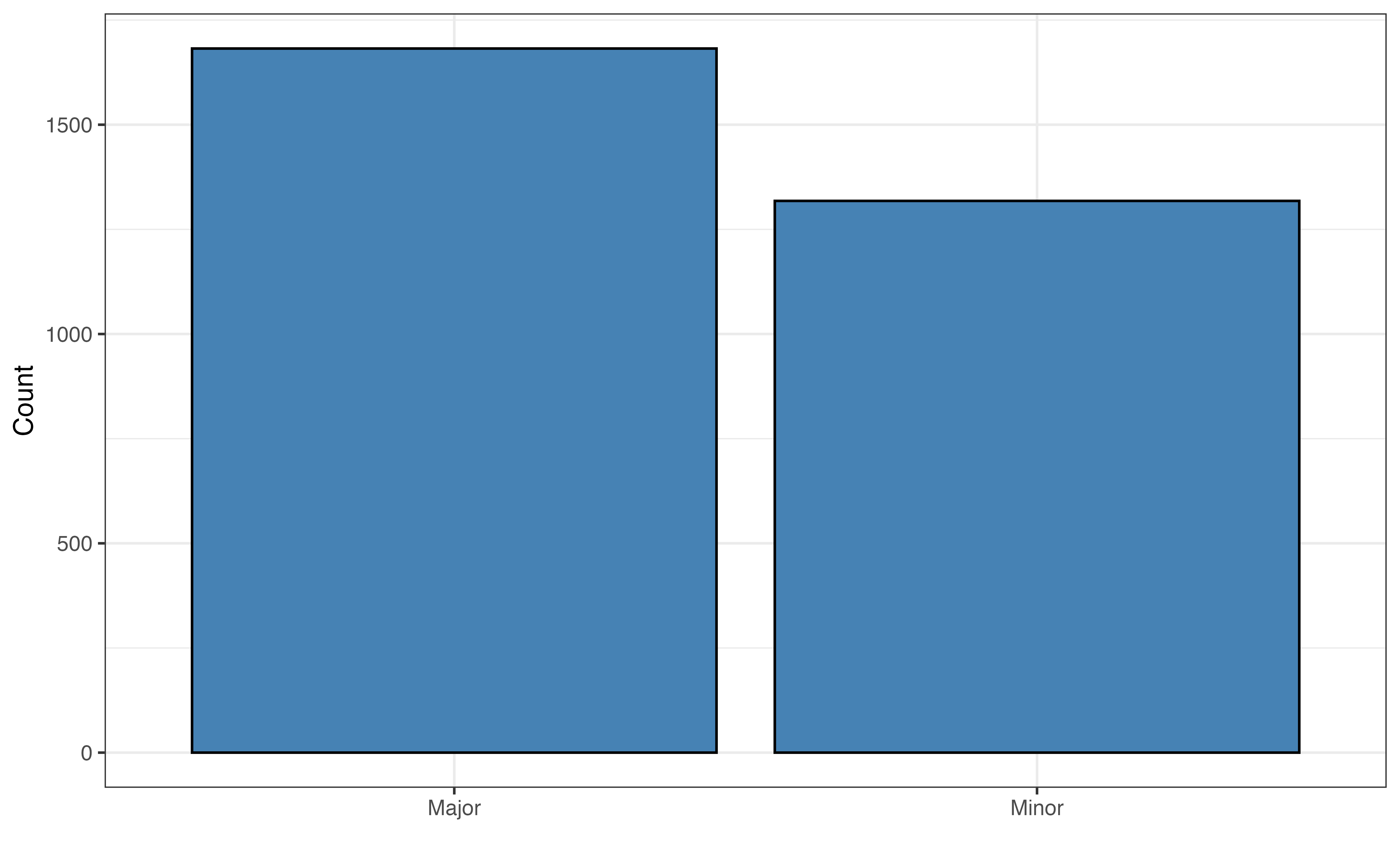
mode: Description of the type of scale for the musical melody of a song. Possible values are “Major” and “Minor”.
acousticness: Measure ranging from 0 to 1 of the confidence a song is acoustic. Values close to 0 are low confidence the song is acoustic, and values close to 1 are high confidence the song is acoustic.
liveness: Measure ranging from 0 to 1 detecting the presence of live audience in the song. Values close to 1 (0.8 or higher) indicate a strong likelihood the song track was recorded in front a live audience.
tempo: Measure of the average pace of a song in beats per minute (BPM).
duration_min: Length of a song in minutes
The goal of this analysis is to explain variability in valence using other musical features. This model can be used for prediction, but the primary objective is explanation.
valence
playlist_genre
danceability
energy
loudness
mode
acousticness
liveness
tempo
duration_min
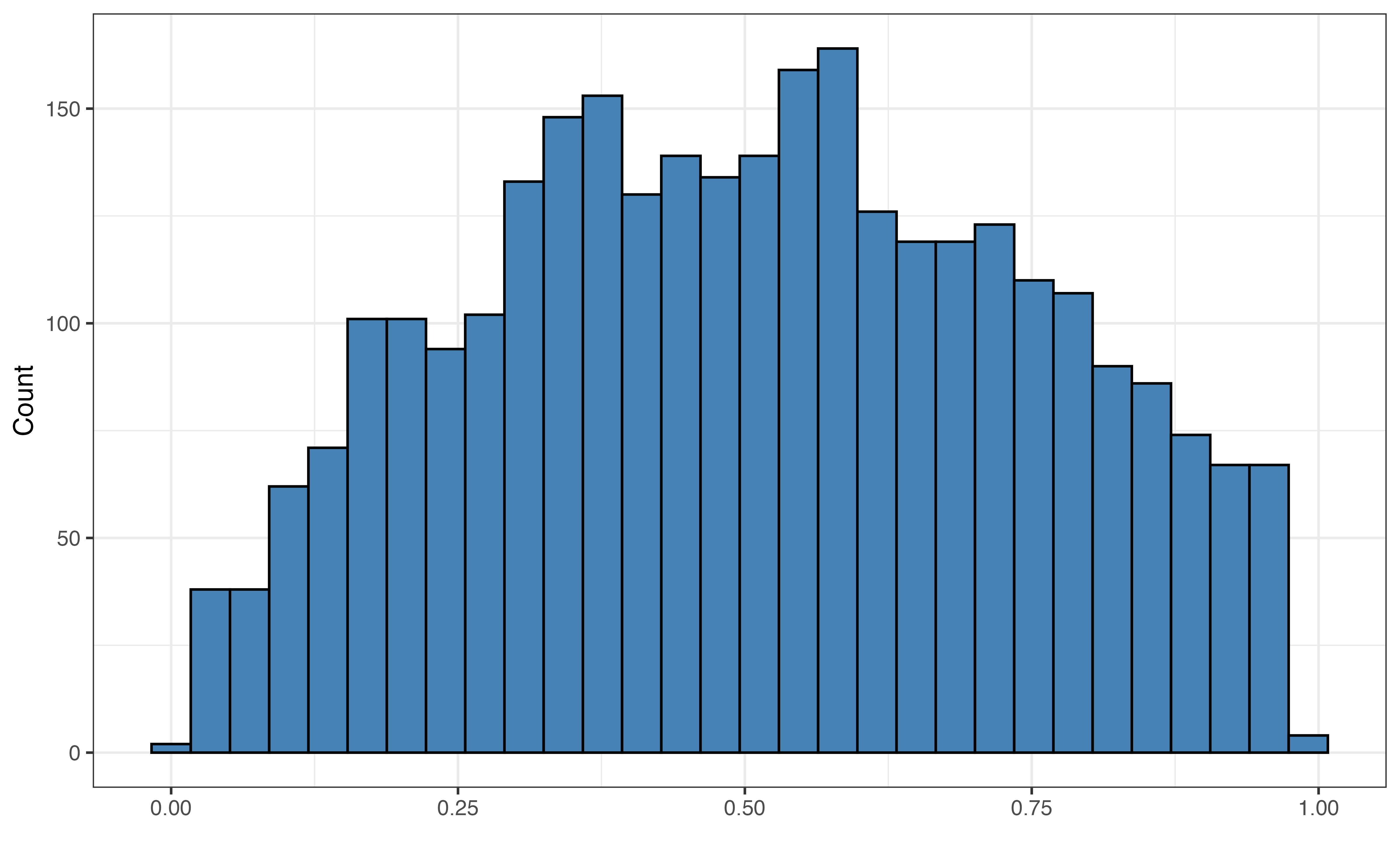
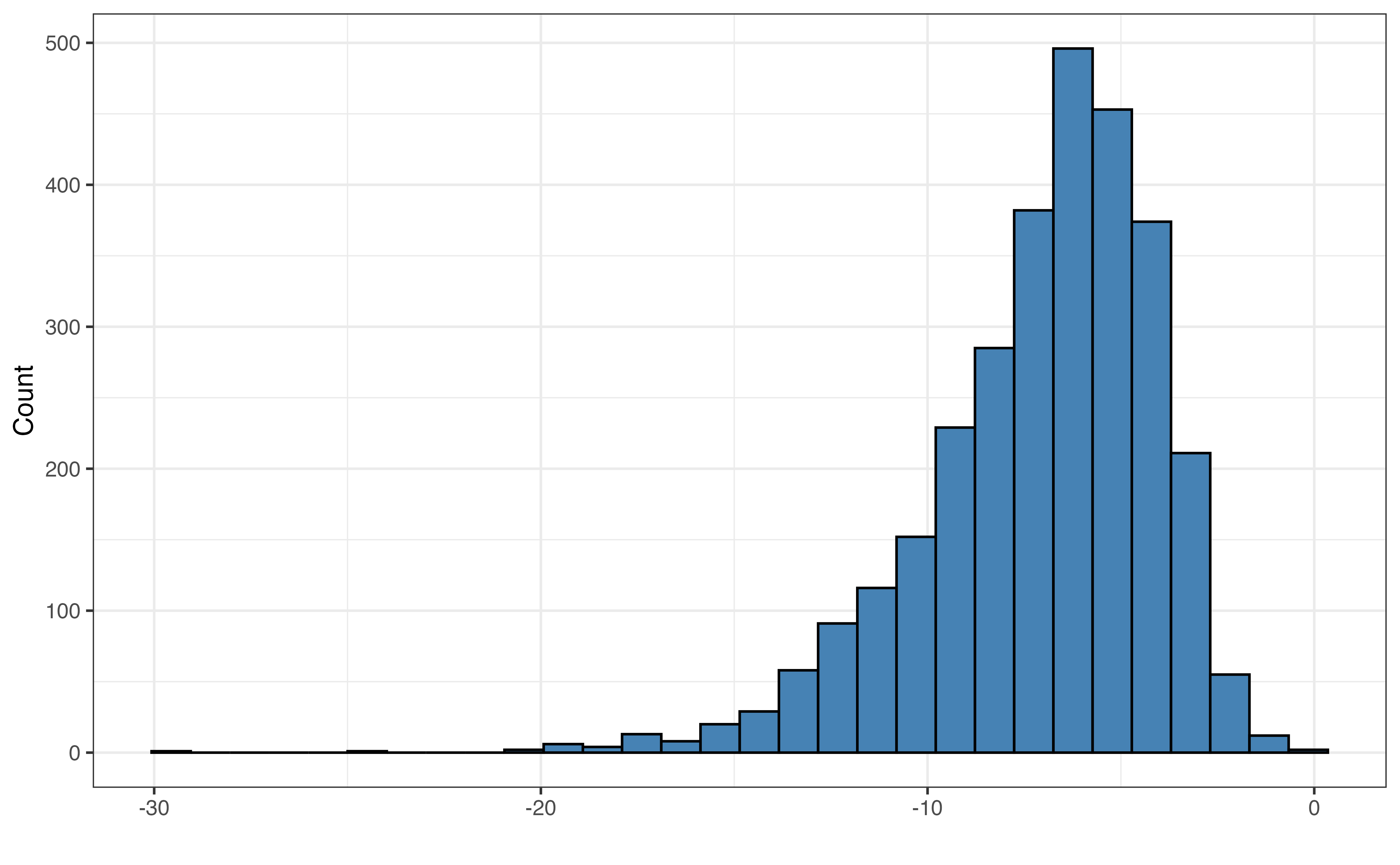
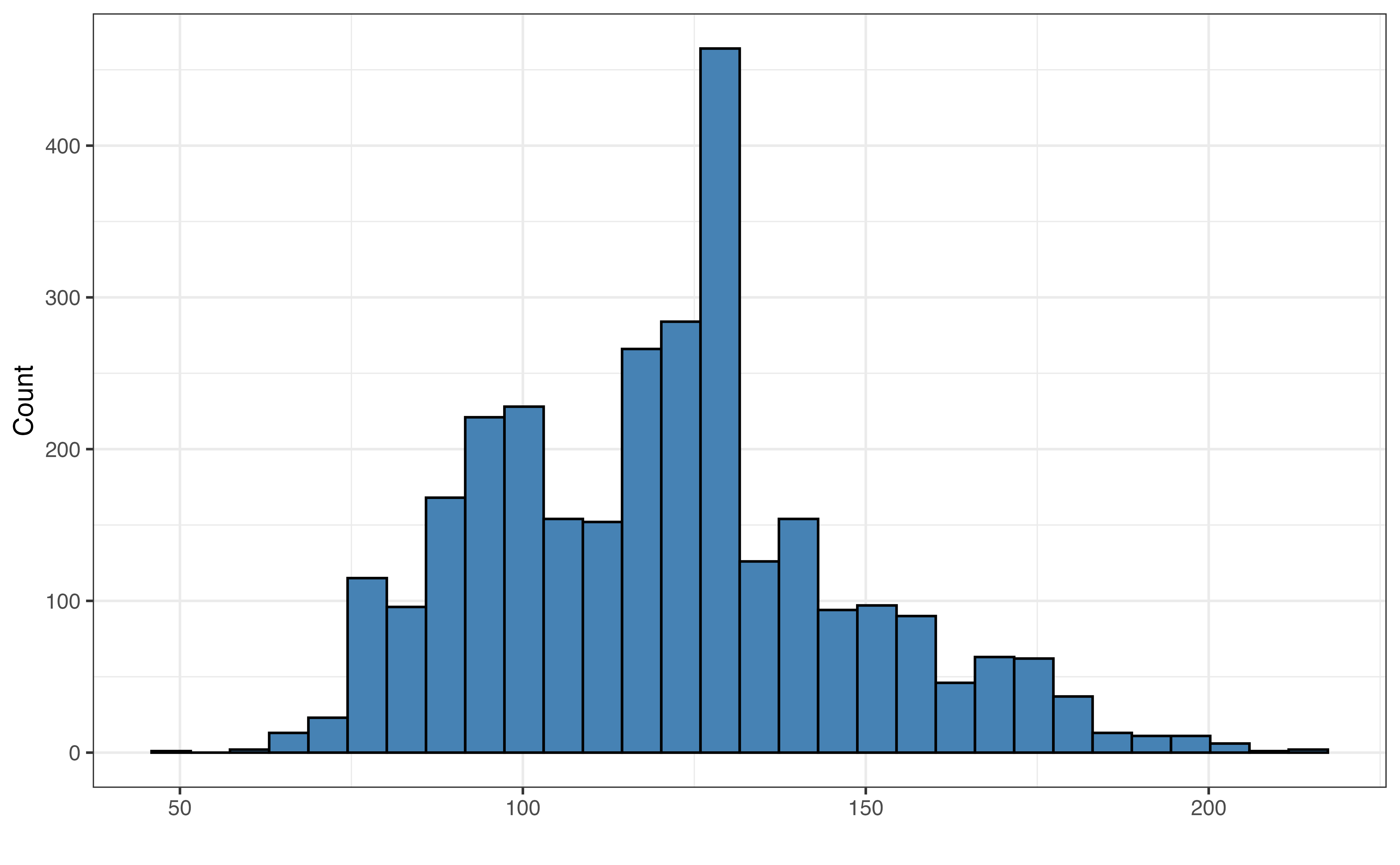
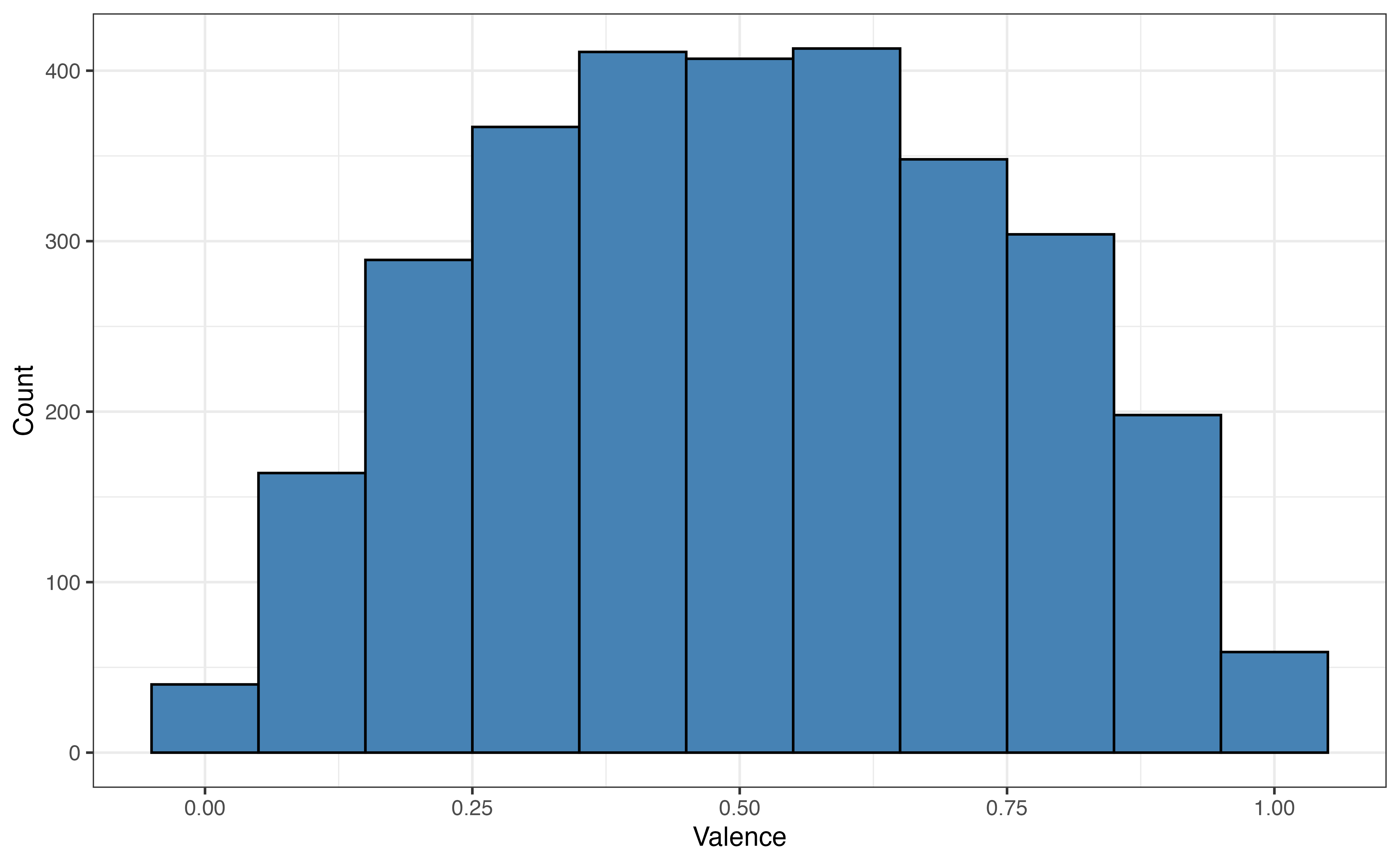
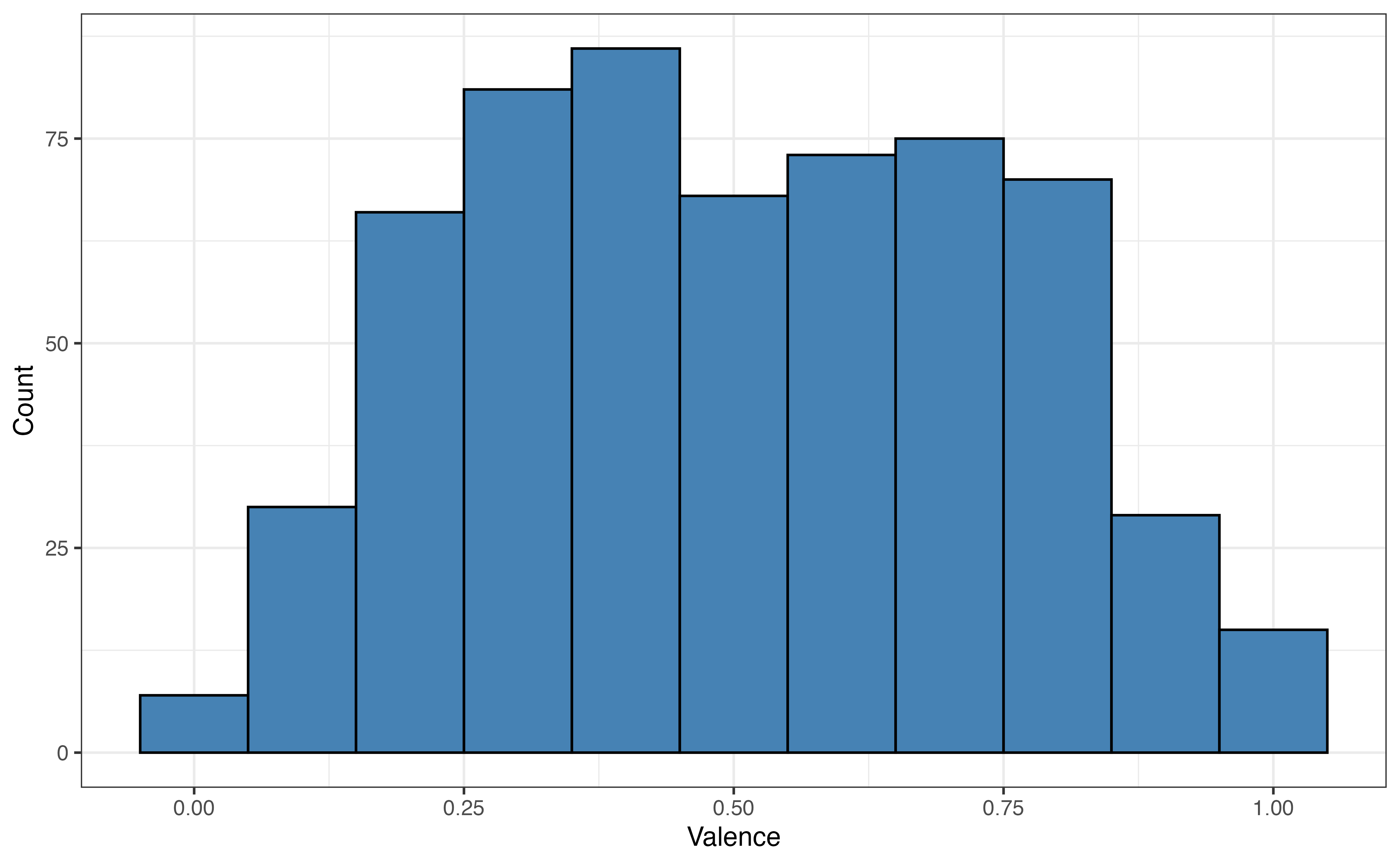
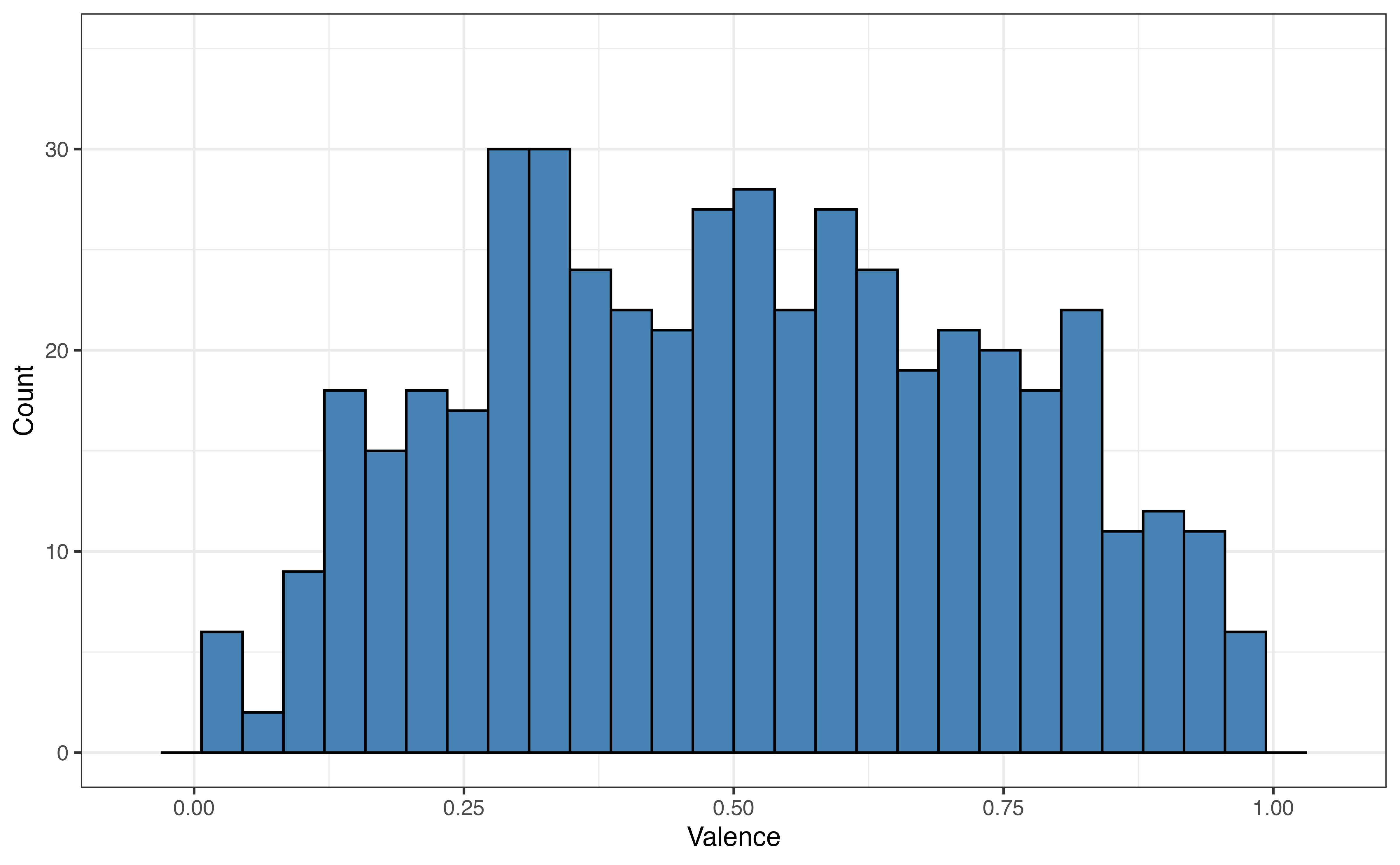
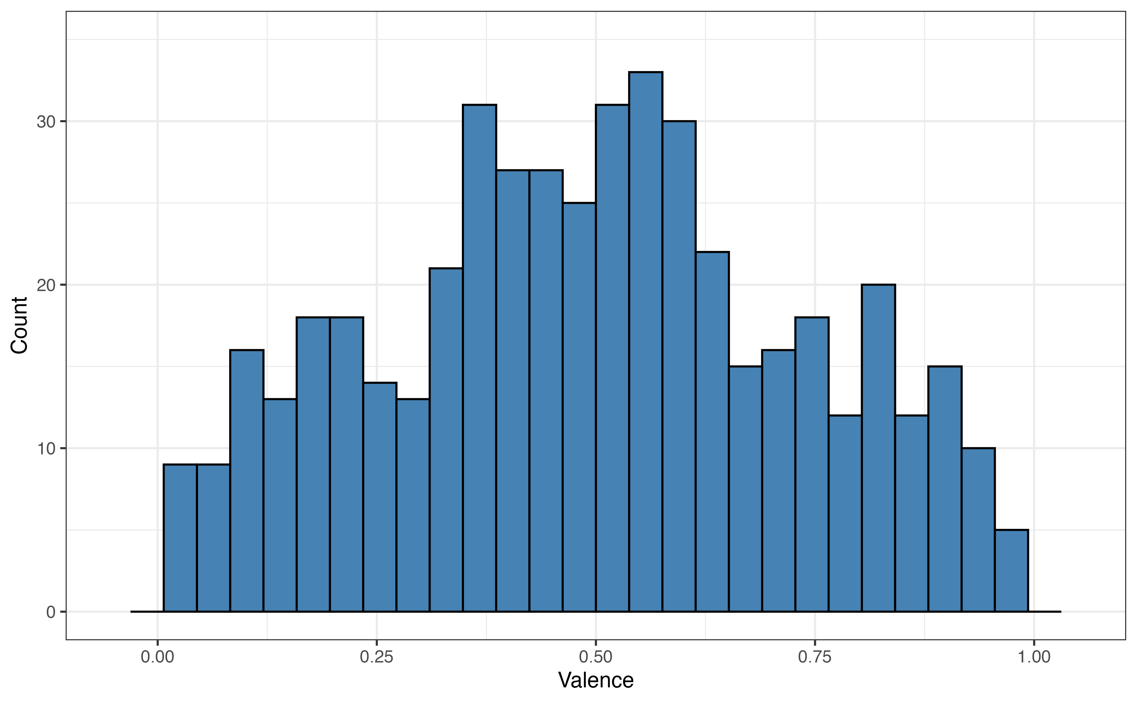
Figure 10.1 (a) shows the distribution of the response variable valence. The distribution is unimodal and approximately symmetric with many songs having values of valence around 0.5 (perhaps indicating a more neutral mood to the song). There is one song that has almost a completely negative mood (valence = 10^{-5}), and one song with an almost completely positive mood (valence = 0.991).
It is worth noting that valence is bounded between 0 and 1, meaning it is not valid to obtain values of valence outside that range. This is not much concern for the purposes of this analysis, because the purpose is primarily explanation. If we intend to build a model whose primary purpose is prediction, then we should more carefully examine any issues and potential transformations for the bounded response variable.
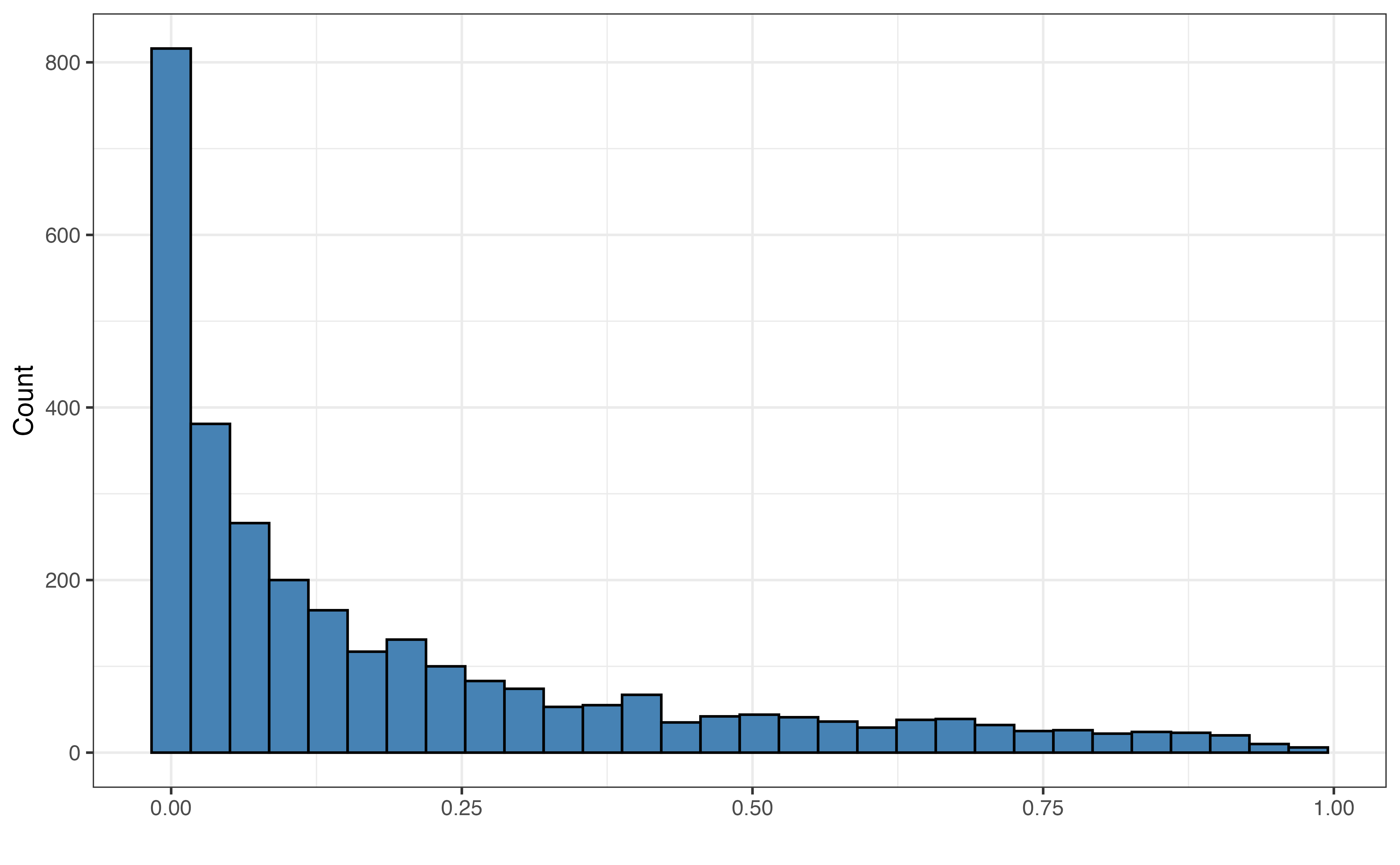
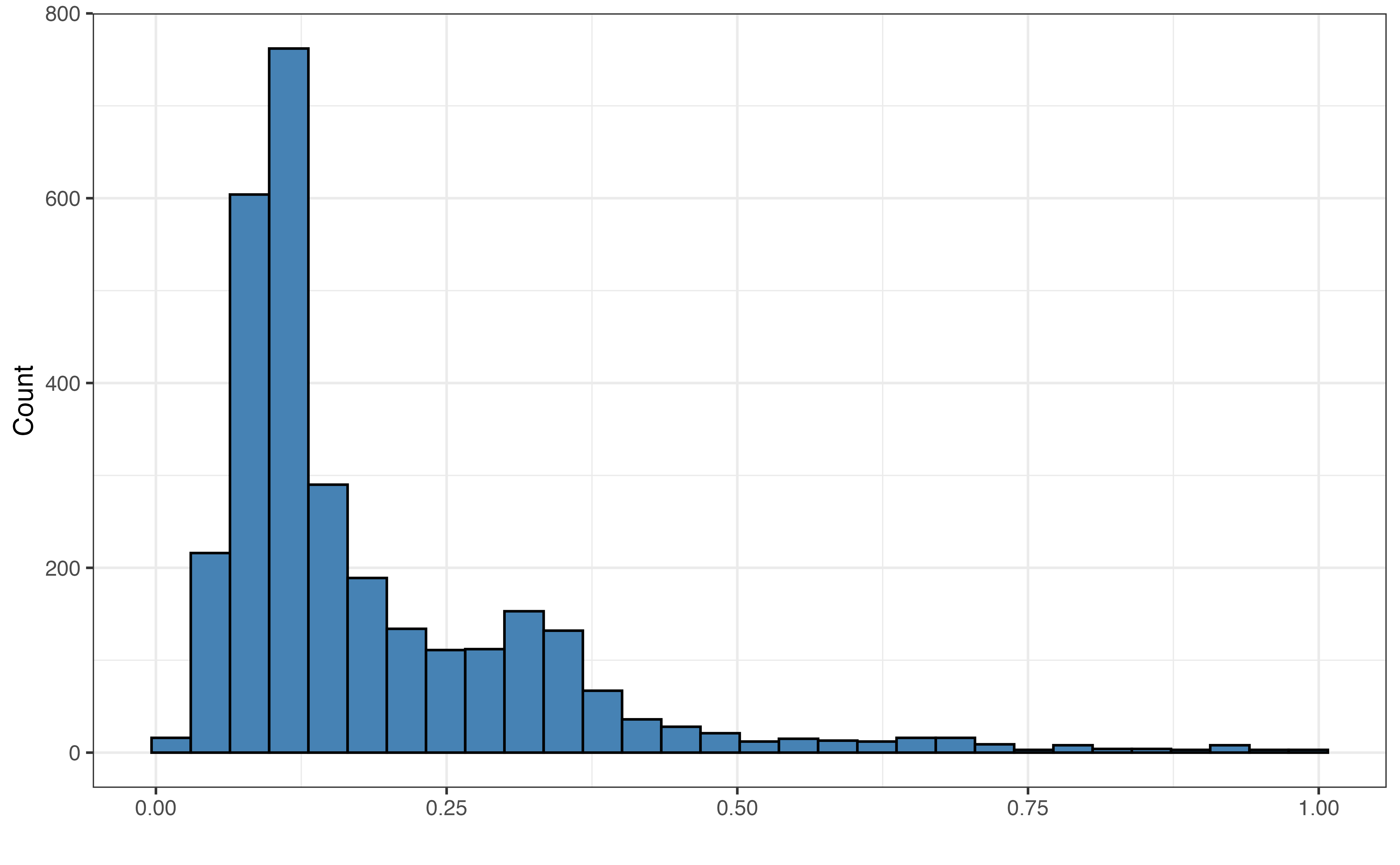
Given the number of potential predictors, we’ll leave observations about the distributions of the predictor variables to the reader.
valence vs. playlist_genre
valence vs. danceability
valence vs. energy
valence vs. loudness
valence vs. mode
valence vs. acousticness
valence vs. instrumentalness
valence vs. liveness
valence vs. tempo
valence vs. duration
valence is on the y-axis.
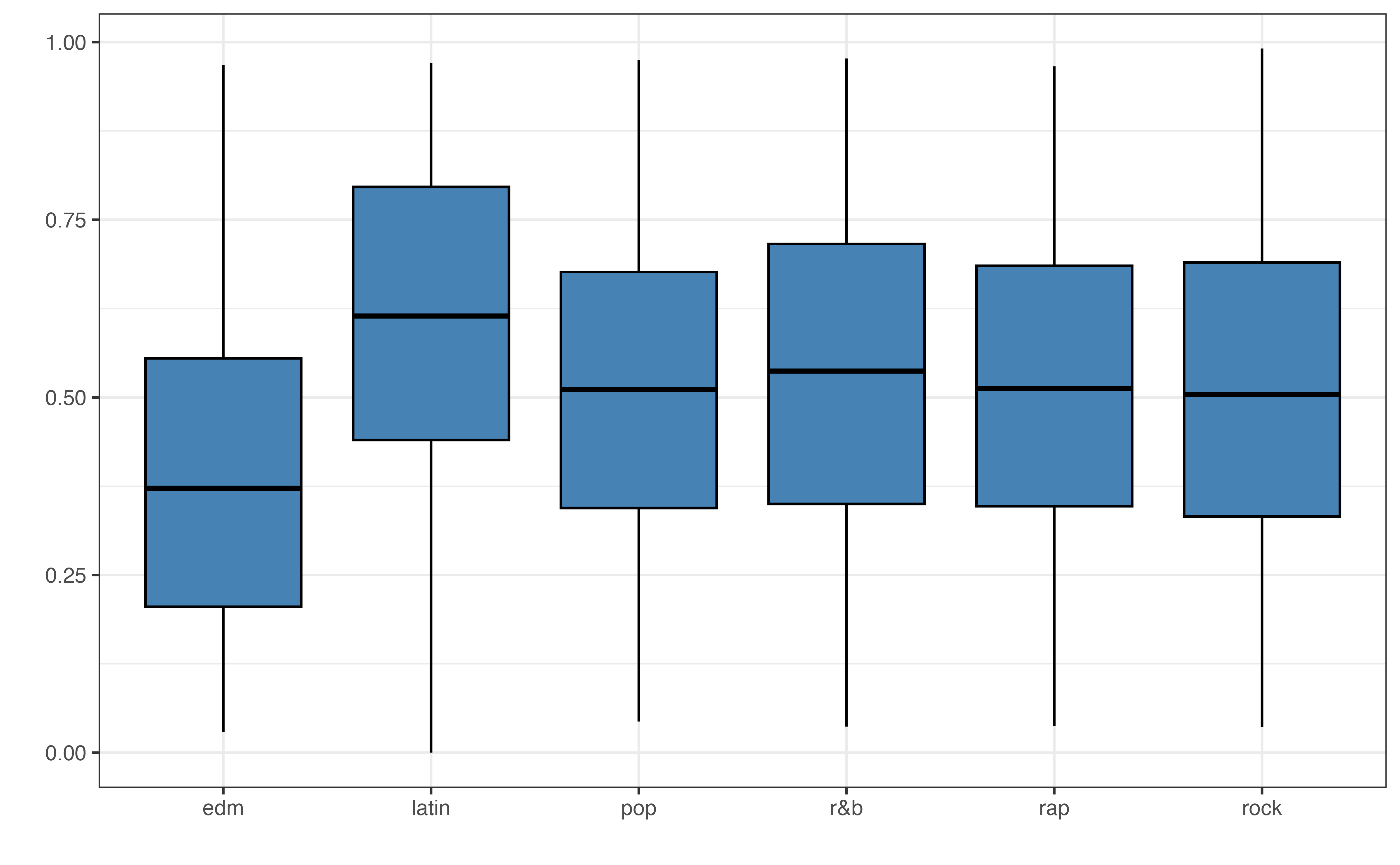
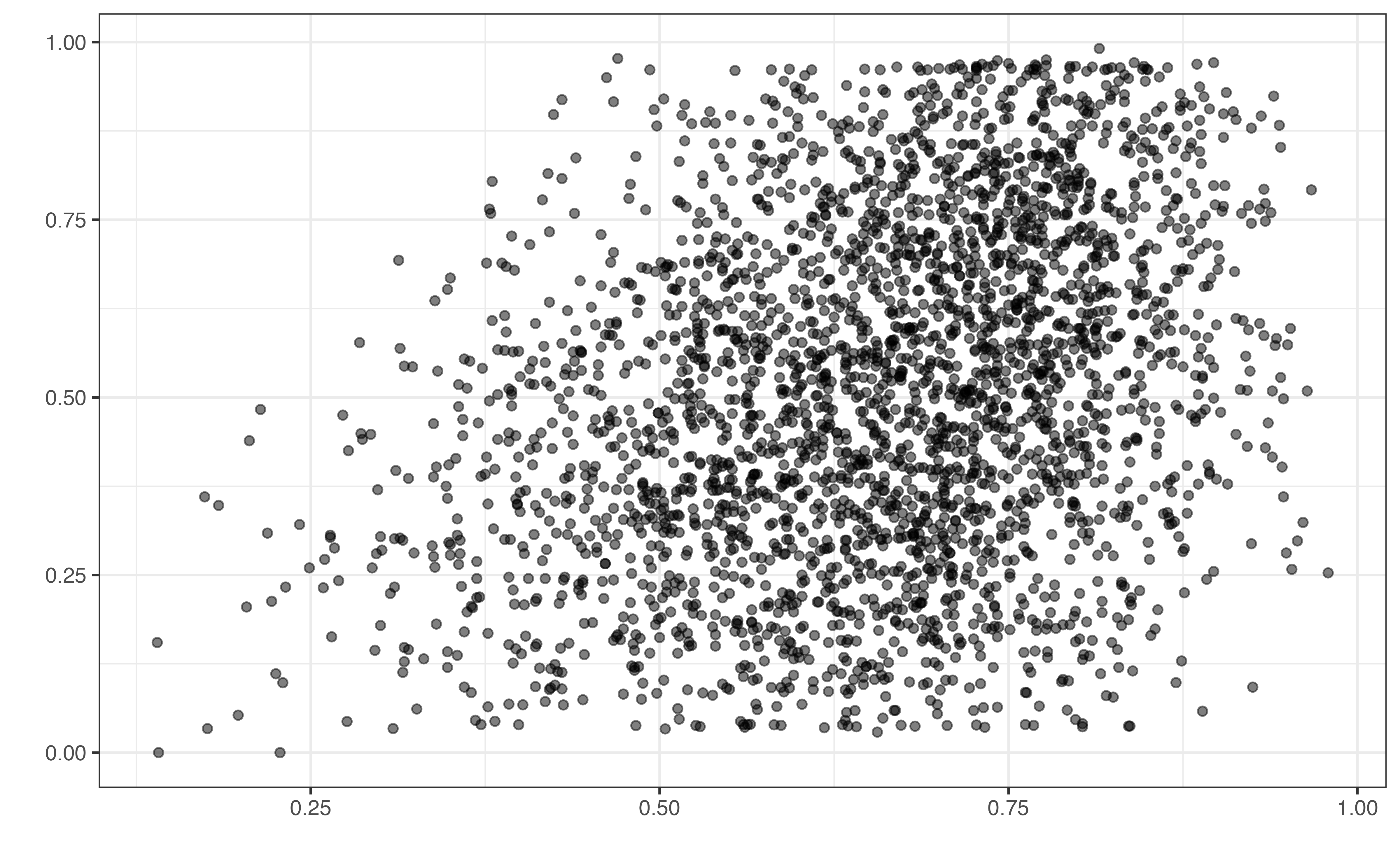
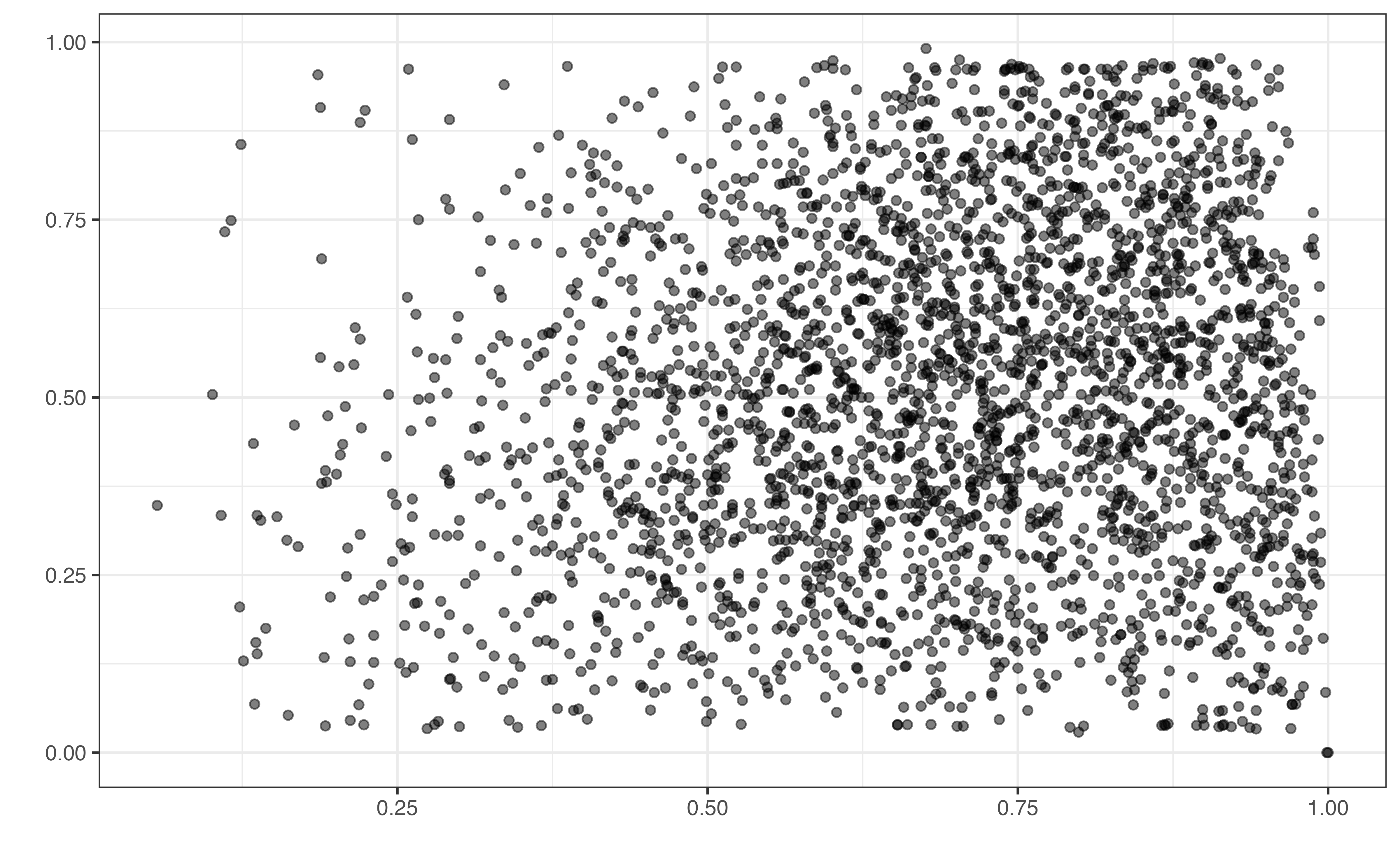
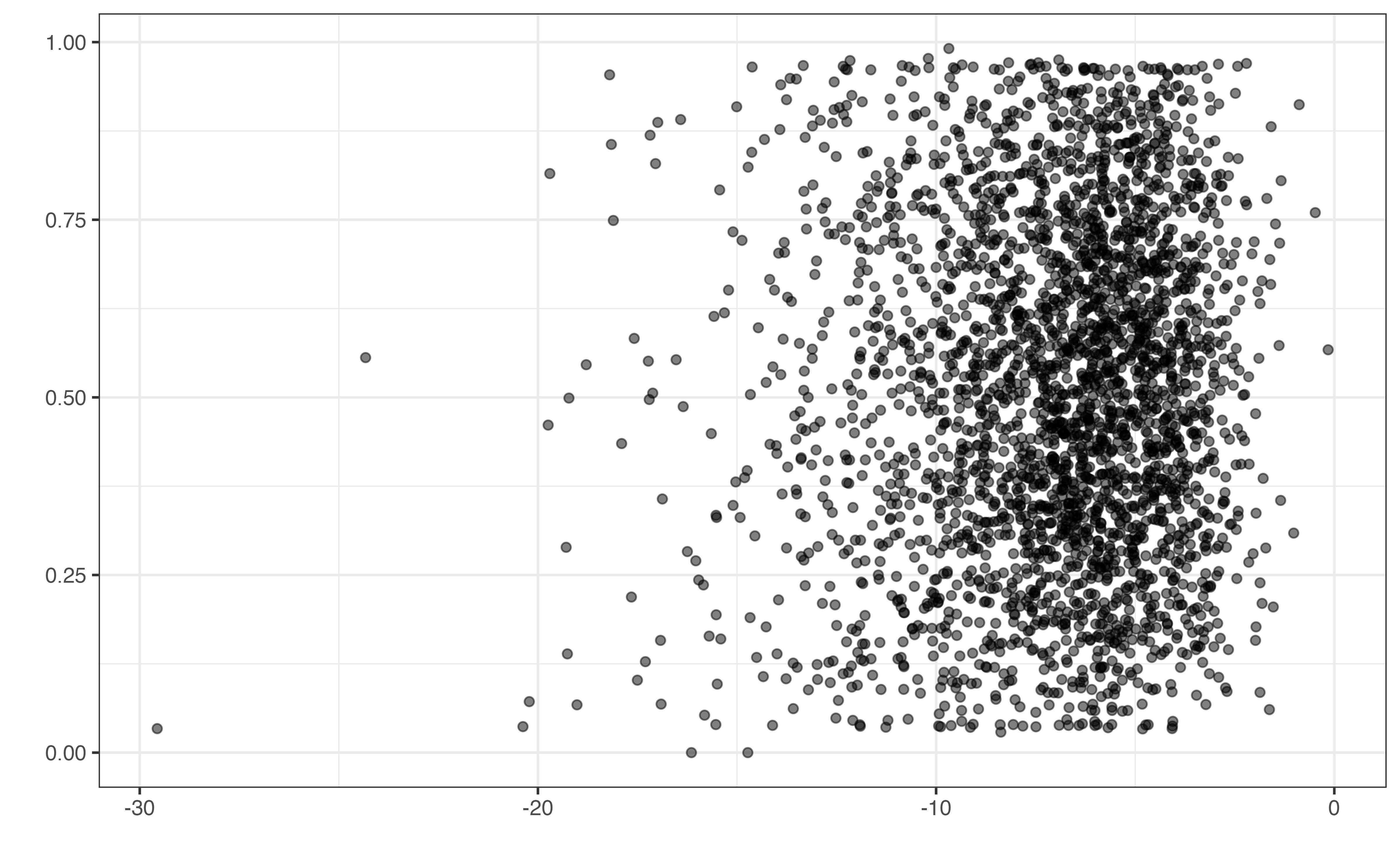
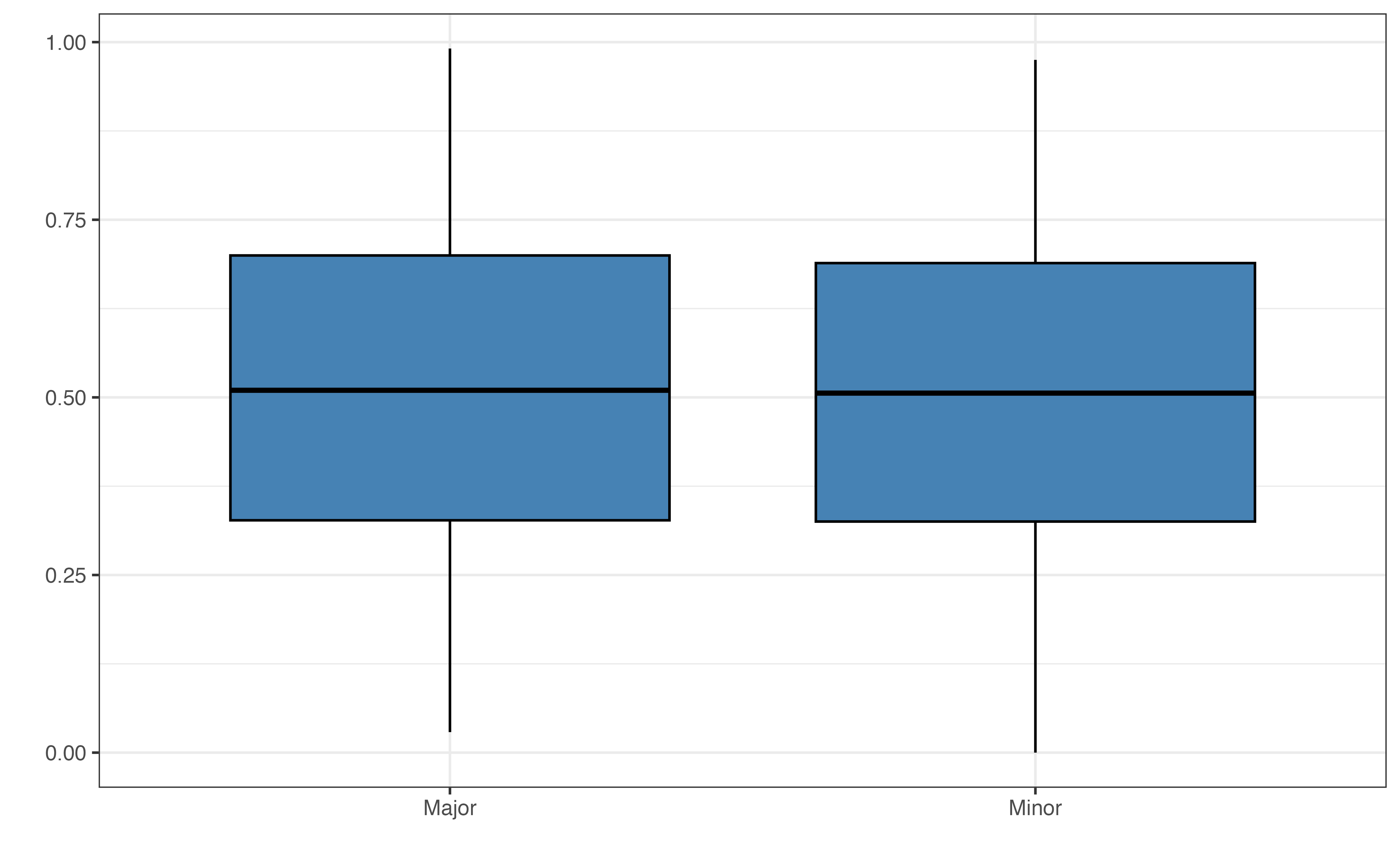
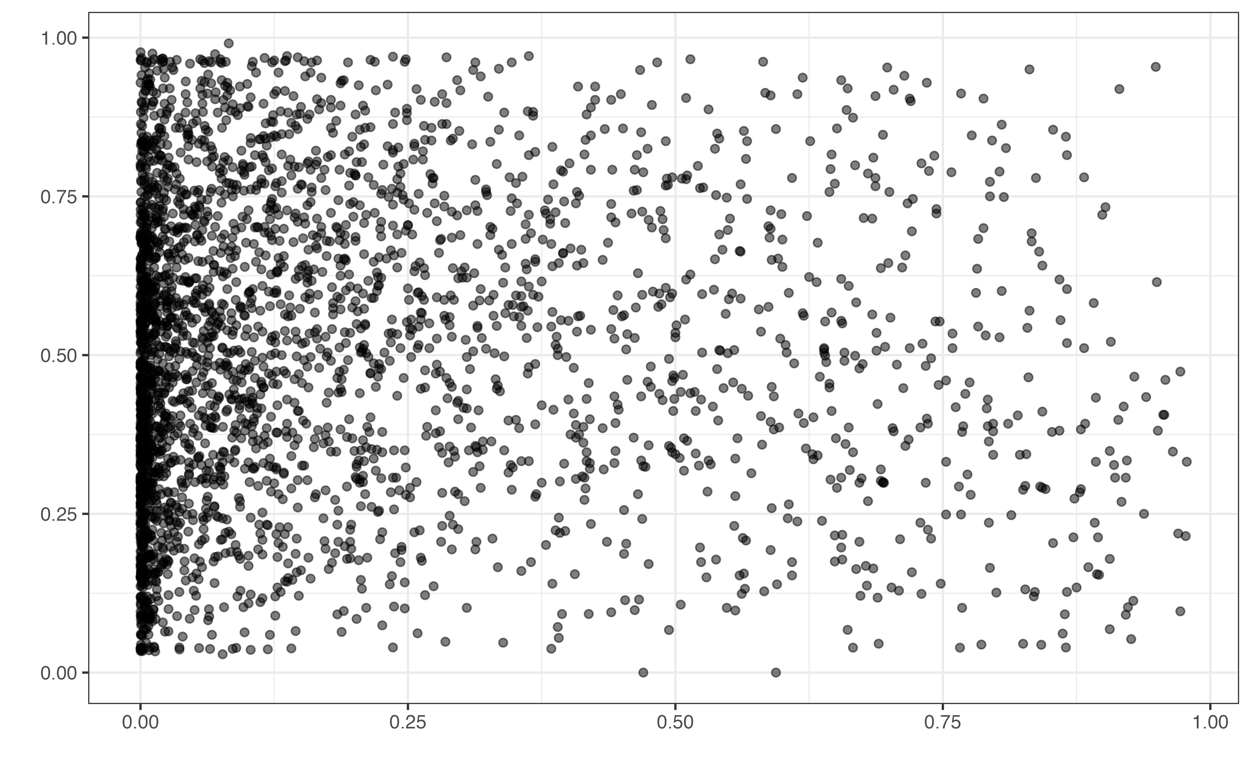
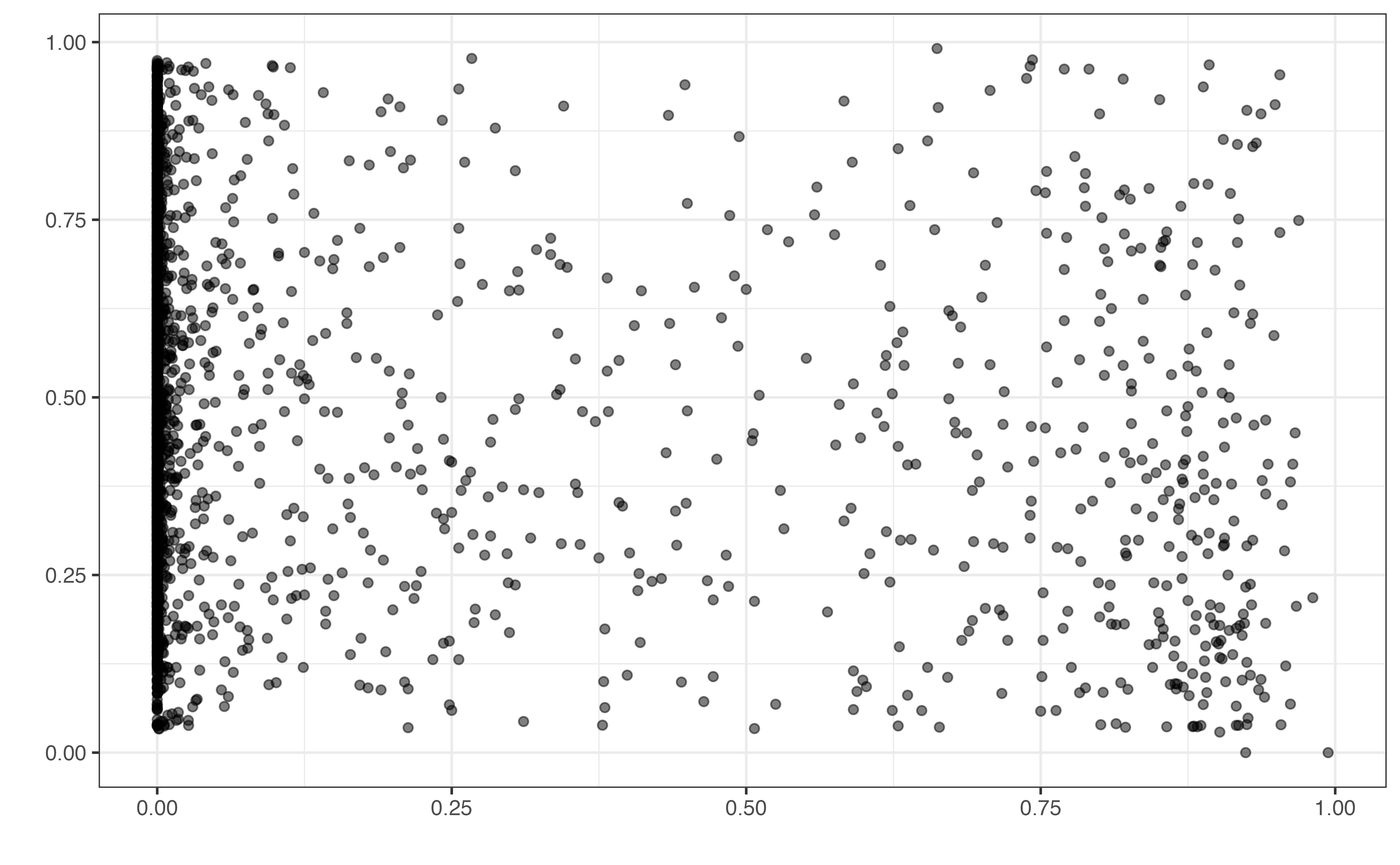
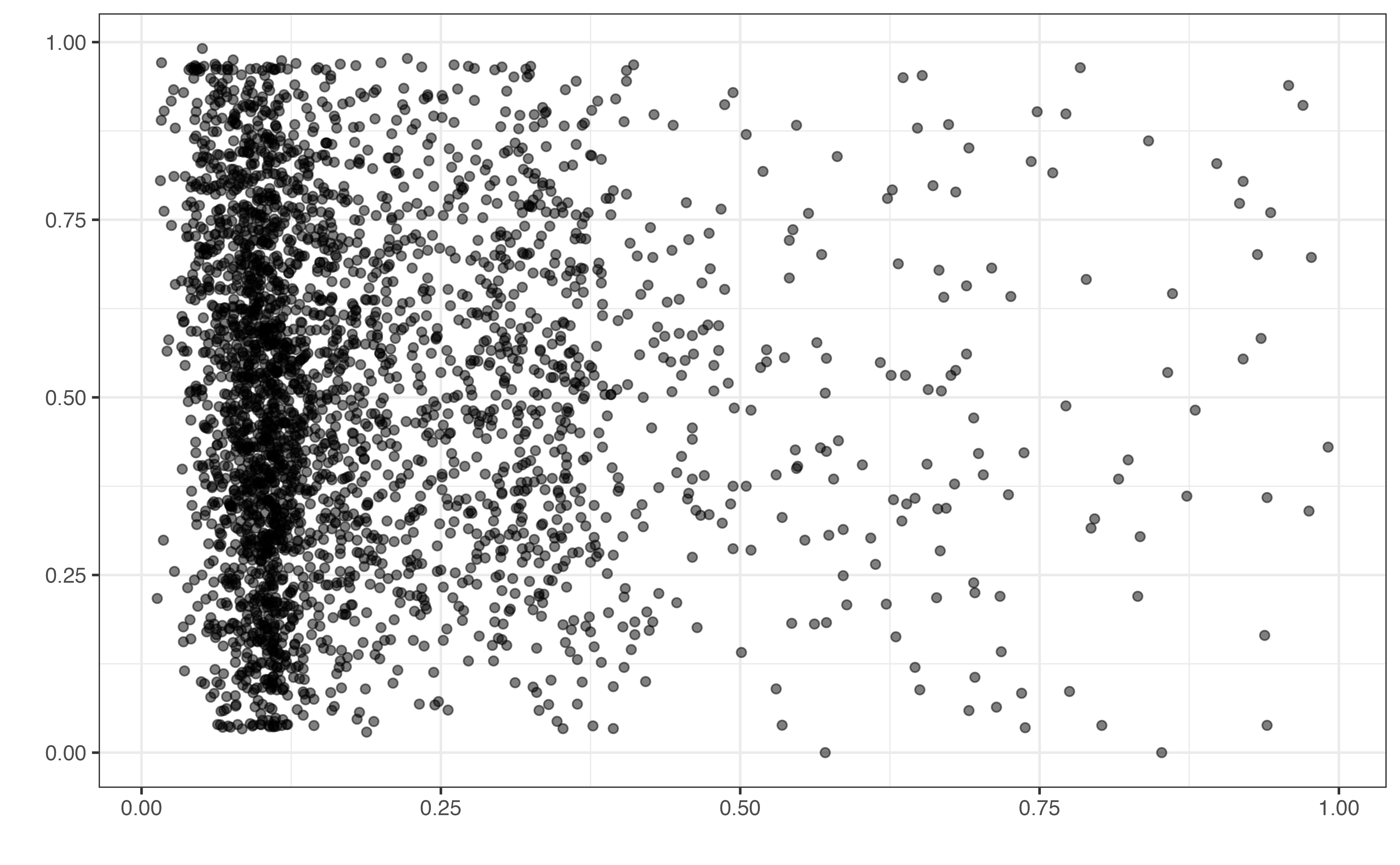
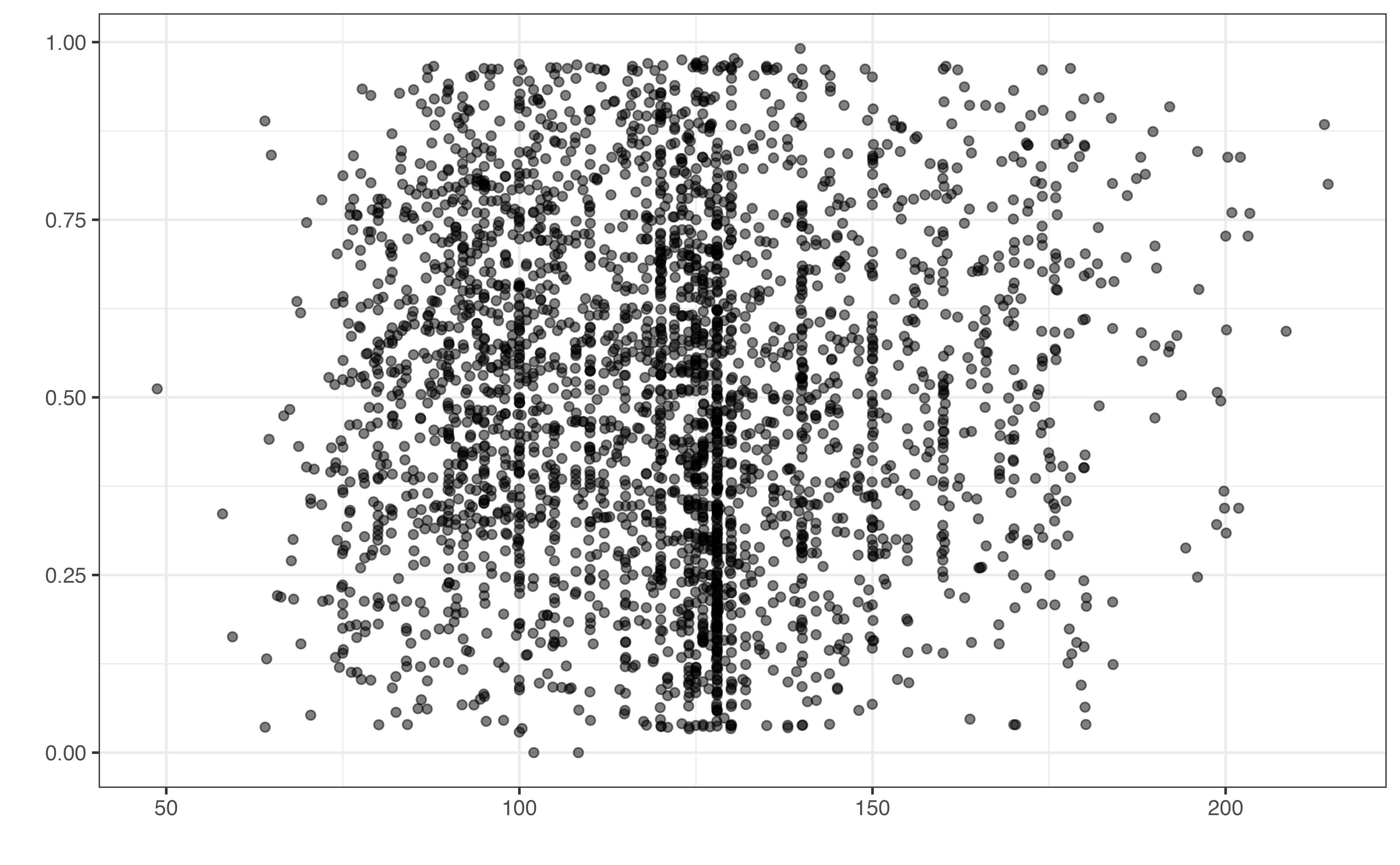
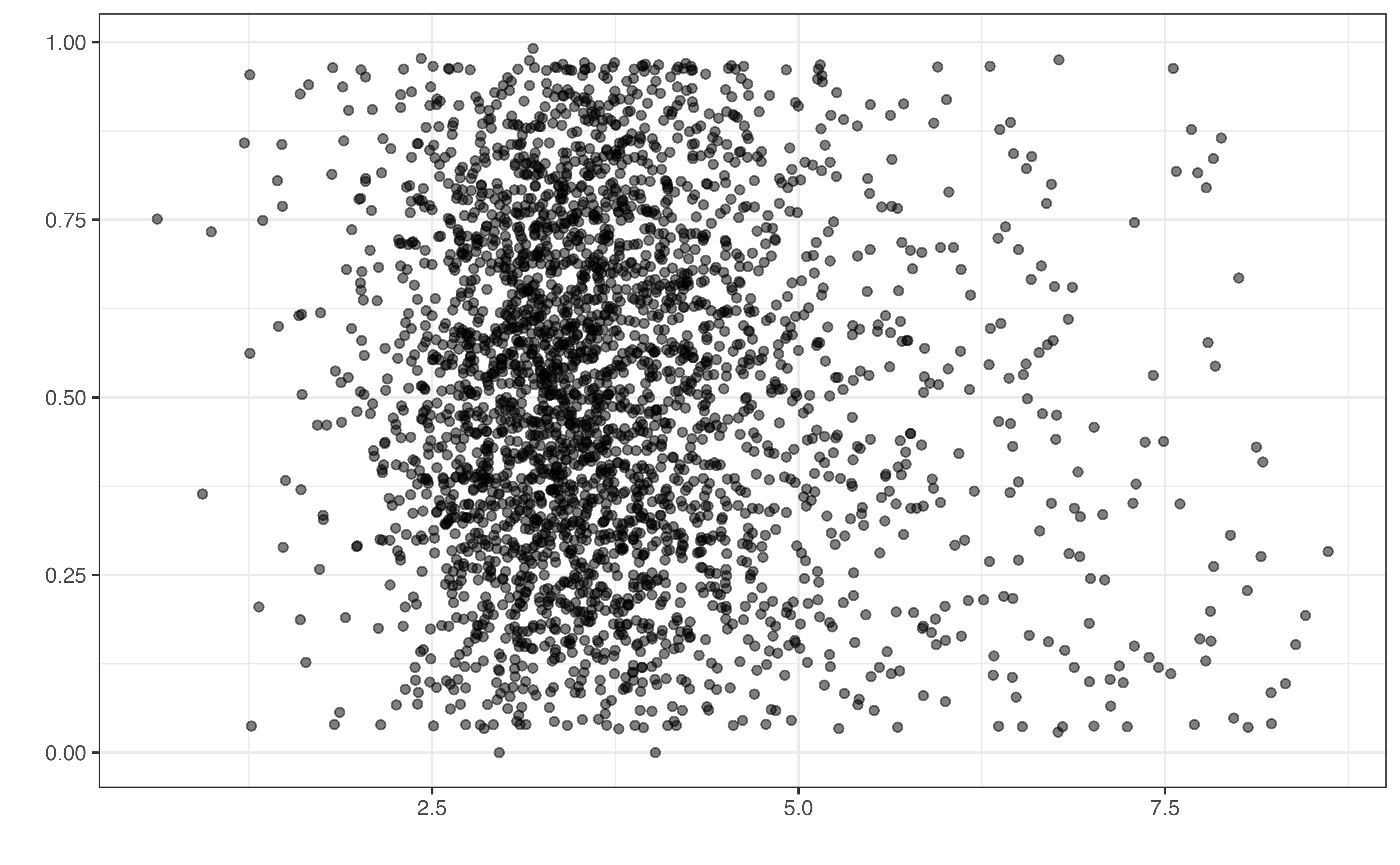
Based on Figure 10.2, which variable(s) do you think have an association with a song’s valence? Describe the direction of the relationship(s).1
Figure 10.2 shows the plots for the bivariate exploratory data analysis. In general, it is more challenging than earlier analyses to see relationships between the valence and the musical features from the bivariate plots. This could be because these features are not actually associated with the valence, or the relationships result from a combination of features rather than individual relationships between each feature and the response. As with previous analyses, the exploratory data analysis is helpful for providing initial intuition about the data and analysis results, but it cannot be used to draw final conclusions. Thus, we choose a model to be used for interpretation and conclusions based on model fit and performance statistics.
In Section 9.5, we compared multiple models to determine which one was the best fit for the data. In these instances, we were comparing models that had the same variables but differed in whether transformations were applied to the response or predictors or whether interactions or higher-order terms were included. Often, however, we do not know which variables to include in the final model and need a way to choose from a set of potential predictors.
When building a regression model, we aim to select the most parsimonious (the simplest) model possible. This means choosing the model with the fewest predictors, interaction terms, and transformations that still effectively summarizes the relationship between the response and predictor variables.
We begin by discussing model fit and performance statistics used to compare models in the model selection process. In Section 4.7, we introduced \(R^2\) and RMSE in to evaluate model fit and predictive performance of regression models. In this section, we introduce new statistics Adjusted \(R^2\), AIC, and BIC, that are also used to compare models. In practice, we often use multiple statistics for model comparison, and sometimes these statistics can suggest we choose different models. Throughout the chapter, we will demonstrate how the analysis objective helps us determine which statistics to prioritize when doing model selection.
Recall from Section 4.7 that \(R^2\) is the proportion of variability in the response variable that is explained by the model. This value is based on the process Analysis of Variance (ANOVA), in which the variability in the response variable is decomposed into variability that can be explained by the model and variability left unexplained in the residuals. Thus, \(R^2\) is computed as
\[ R^2 = \frac{SSM}{SST} = 1 - \frac{SSR}{SST} \tag{10.1}\]
where \(SSM\) is the model sum of squares (explained variability), \(SSR\) is the residual sum of squares (unexplained variability), and \(SST\) is the total variability in the response variable.
Thus far, we have used \(R^2\) to describe how well a model fits the data and to compare two models with the same number of predictors (for example, in Section 9.5). Now as we prepare to do model selection, we will often be comparing models that have different numbers of predictor variables, since the model selection process is often us answering the question “should we include predictor \(X_j\) in the model given the other predictors currently in the model?”. Recall from Section 7.3 that the coefficients for a least-squares regression model are the ones that minimize the sum of square residuals (\(SSR\)). Thus, if we estimate non-zero coefficients for new predictors, \(SSR\) will decrease (even if it’s just by a very small amount) by definition. Thus, we cannot use \(R^2\) to compare models with different numbers of predictors, because \(R^2\) tends to preference the model with more predictors. This can lead to overfitting, the case in which a model fits so closely to the sample data that it cannot be reliably used on new data.
When comparing models with different numbers of predictors, we can use a related statistic, called Adjusted\(R^2\) that takes into account the number of predictor variables in the model.
The formula for Adjusted \(R^2\) is
\[ \text{Adjusted }R^2 = 1 - \frac{SSR / (n - p - 1)}{SST / (n - 1)} \tag{10.2}\]
where \(SSR\) and \(SST\) are defined as before, \(n\) is the number of observations in the data, and \(p\) is the number of predictors.
The numerator \(SSR / (n - p - 1)\), the residual sum of squares divided by the associated degrees of freedom, is a measure of the average variability about the regression line. We showed in Section 8.4.1 that the regression standard error, \(\hat{\sigma} = \sqrt{\frac{SSR}{n - p -1}}\), is the square root of this value. The variability about the regression line will be smaller for models that are a better fit for the data. Thus, \(SSR / (n - p - 1)\) will decrease only if adding new predictors makes the model a better fit for the data.
The denominator, \(SST/(n-1)\), is the sum of squares total divided by the associated degrees of freedom. This is the variance of the response variable, \(s^2_{Y}\) . It will remain the same for all candidate models, because the same sample data is used throughout the analysis.
Putting what we know about the numerator and denominator together, the second term in the Equation 10.2 is smaller for models that better fit the data. Therefore, the Adjusted \(R^2\) will be greater for models that are a better fit. Adjusted \(R^2\) ranges from 0 to 1, so we choose models that have values close to 1.
The degrees of freedom (df) are the number of observations available to understand variability.
When we fit a regression line with \(p\) predictors, we need a minimum of \(p + 1\) observations to fit the line, where \(p+1\) is the number of terms in the model (including the intercept). We are left with \(n - (p + 1) = n - p - 1\) observations to understand any variability in the residuals about the line. Thus, the degrees of freedom associated with SSR is \(n - p - 1\).
The degrees of freedom associated with \(SST\) are the number of observations needed to understand variability about the mean of the distribution of the response variable. We need a minimum of one observation to compute a mean, so we are left with \(n - 1\) observations to understand variability about the mean.
Let’s look at an example of two candidate models to explain a song’s valence. The first model includes the predictor danceability, and the second model includes the predictors danceability, mode, and liveness.
valence
| Model | R-sq | Adj. R-sq |
|---|---|---|
| Danceability | 0.0957 | 0.0954 |
| Danceability, Mode, Liveness | 0.0960 | 0.0951 |
From Table 10.1, we see the model fits are very similar. Though \(R^2\) is slightly higher for the model with the additional predictors mode and liveness, Adj. \(R^2\) is higher for the model that only includes danceability . This means that adding mode and liveness to the model dose not explain much additional variability in a song’s valence after accounting for danceability. Thus, we might prefer the model that only contains danceability given the goal of choosing of the simplest model possible that is still effective.
Below are guidelines for using \(R^2\) and Adjusted \(R^2\) in practice.
\(R^2\)
Adjusted \(R^2\)
Another statistic for model comparison is the Root Mean Square Error introduced in Section 4.7. The Root Mean Square Error (RMSE) is a measure of the average error in the model predictions. From Equation 10.3, we can see it is very similar to \(\hat{\sigma}\) (Equation 8.3). In fact, the difference between these values is negligible when the number of observations, \(n\), is large.
\[ RMSE = \sqrt{\frac{\sum_{i=1}^n(y_i - \hat{y}_i)^2}{n}} = \sqrt{\frac{SSR}{n}} \tag{10.3}\]
The RMSE is typically used over other model comparison statistics, such as Adjusted \(R^2\), when the primary modeling objective is prediction.
We use RMSE to compare two models. In general, do we select the model with the higher or lower value of RMSE?2
Table 10.2 shows the RMSE for the two models compared in Section 10.2.1.
| Model | RMSE |
|---|---|
| Danceability | 0.225 |
| Danceability, Mode, Liveness | 0.225 |
Recall that RMSE has the same units and scale as the response variable, so we take these into consideration when interpreting RMSE and using it to compare models. Based on Table 10.2, the values of RMSE for the two models are equal down to three digits. From Section 10.1, valence takes values 0 to 1, so a difference less than 0.001 in the prediction error is very small. This is consistent with the very small difference in Adjusted \(R^2\) values in Table 10.1. In general, we select the model that has the smallest value of RMSE; however, in cases like this with negligible to no difference between the two models, we use our judgment as the data scientist, along with subject matter expertise and the analysis objectives to choose a model.
Adjusted \(R^2\) and RMSE are computed by quantifying the variability in the residuals (the unexplained variability). In addition to these statistics are two other statistics, AIC and BIC, that are based on another measure of model fit called a likelihood function. We will talk about the likelihood in more detail in Chapter 11, but in short, a likelihood function quantifies how plausible it is to obtain the observed data given a particular model is the true model of the relationship between the response and predictor variables. Models with higher values for the likelihood are a better fit for the data compared to models with lower values. It is common to work with the natural log of the likelihood function, denoted \(\log L\), for ease of calculations. The natural log is monotonic, so higher values of \(\log L\) correspond to higher values of the likelihood and vice versa.
The Akaike’s Information Criterion (AIC) (Akaike 1974) and Schwarz’s Bayesian Information Criterion (BIC) (Schwarz 1978) are two measures of model fit based on the likelihood. Their equations are
\[ \begin{aligned} AIC &= -2\log L + 2(p+1) \\ BIC &= -2\log L + \log(n)(p+1) \end{aligned} \tag{10.4}\]
where \(\log L\) is the log-likelihood, \(n\) is the number of observations, and \(p+1\) is the number of terms in the model.
In Equation 10.4, the first term for both AIC and BIC is \(-2 \log L\). Because the log-likelihood is greater for better fitting models, this term decreases as the model fit improves. The second term in each equation is the “penalty” for the number of predictors in the model. As new predictors are added to a model, AIC and BIC are a balance between the decreasing first term and increasing second term. Where AIC and BIC differ is on the strength of the penalty for the number of terms in the model. When \(n > 8\) (essentially all the time!), \(\log(n)(p+1) > 2(p + 1)\), so we say BIC has the “stronger penalty”. This results in BIC tending to preference models with fewer predictor variables than AIC.
The AIC and BIC for a single model is generally not meaningful in practice, so these values are used to compare two or more models. Small values of AIC and BIC correspond to better model fit, so we select the model that minimizes these statistics when comparing multiple models. In practice, a difference of 10 or greater in the AIC or BIC between models, is considered meaningful enough to choose one model over the other. Table 10.3 provides more specific guidelines for model comparison based on the differences in AIC and BIC.
Below are the values of AIC and BIC from the candidate models introduced in Section 10.2.1.
| Model | AIC | BIC |
|---|---|---|
| Danceability | -427 | -409 |
| Danceability, Mode, Liveness | -424 | -394 |
Using Table 12.8, which model would you choose based on AIC? Based on BIC? 5
In this example, the same model minimizes both AIC and BIC. In fact, based on the guidelines in Table 10.3, the difference in the values of BIC provides very strong support of the model that only includes danceability. Sometimes, a model may have the minimum value of AIC but not have the minimum value of BIC or vice versa. Thus, we can choose which statistic to prioritize based on the analysis objective. If the primary objective is explanation, the model selected by AIC is preferred, because AIC tends to choose the model with more variables that can help explain variability in the response. If the primary objective is prediction, the model selected by BIC is preferred, because BIC selects the model with fewer predictors, thus reducing the variability in the model predictions.
Model comparison statistics
Below is a summary of the model comparison statistics:
| Statistic | Equation | Values that indicate good fit | Prioritize when analysis objective is… |
|---|---|---|---|
| Adjusted \(R^2\) | \(\frac{SSR/ (n - p - 1}{SST / (n - 1)}\) | Higher | Explanation |
| RMSE | \(\sqrt{\frac{SSR}{n}}\) | Lower | Prediction |
| AIC | \(-2\log L + 2(p+1)\) | Lower | Explanation |
| BIC | \(-2\log L + \log(n)(p+1)\) | Lower | Prediction |
Now that we have a suite of model comparison statistics, let’s develop a workflow for using these statistics to choose a final model. In Section 10.2, we compared two models with a small number of predictor variables. From Section 10.1, we see there are nine potential predictor variables. Even with nine potential predictors, it would be time consuming and computationally intensive to test every possible combination of predictors. In practice, we may even have as many as 20, 50, or many more predictors to consider for inclusion in a model. Therefore, we need methods that help us choose variables to include in the model in a systematic way. This is called model selection.
In particular, we will use a set of methods called stepwise selection, where were considering adding and/or removing one variable or a small subset of variables at a time (the steps).
The first stepwise method is forward selection. In forward selection, we begin with the intercept-only model (also called the null model), and add variables one at a time until we can no longer find a model that is a better fit than the current one. We use the model comparison statistics from Section 10.2 to determine the variables to add to the model. The steps for forward selection are as follows:
Start with the intercept-only model, then for each step:
Let’s look at an example of forward selection using AIC to compare the models. In the first step, the “current” model is the intercept-only model. We compute AIC for this model and all possible models with a single predictor. Table 10.6 shows the results in order of AIC.
valence ~ 1 is the intercept-only model.
| Candidate model | AIC |
|---|---|
| valence ~ danceability | -427 |
| valence ~ playlist_genre | -343 |
| valence ~ energy | -179 |
| valence ~ duration | -146 |
| valence ~ loudness | -136 |
| valence ~ liveness | -127 |
| valence ~ 1 | -127 |
| valence ~ mode | -125 |
| valence ~ tempo | -125 |
| valence ~ acousticness | -125 |
Based on AIC, a model with danceability is the best model out of the current candidates. Therefore, as forward selection progresses, we limit the space of candidate models to those that include danceability as a predictor. Table 10.7 shows the next step of forward selection. We compute AIC for all two-predictor models that have danceability as one of the predictors, along with the current model that only has danceability as a predictor.
| Candidate model | AIC |
|---|---|
| valence ~ danceability + playlist_genre | -709 |
| valence ~ danceability + energy | -508 |
| valence ~ danceability + loudness | -439 |
| valence ~ danceability + duration | -438 |
| valence ~ danceability + tempo | -432 |
| valence ~ danceability | -427 |
| valence ~ danceability + mode | -425 |
| valence ~ danceability + liveness | -425 |
| valence ~ danceability + acousticness | -425 |
Based on Table 10.7, we choose the model that includes danceability and playlist_genre, because it is the model that minimizes AIC. Now, as we continue with forward selection, the space of potential models is narrowed to those that have danceability and playlist_genre as predictors. This process is continued until adding a new predictor to the model does not improve model fit based on AIC.
| term | estimate | std.error | statistic | p.value |
|---|---|---|---|---|
| (Intercept) | -0.423 | 0.046 | -9.16 | 0.000 |
| danceability | 0.639 | 0.029 | 21.88 | 0.000 |
| playlist_genrelatin | 0.203 | 0.013 | 15.90 | 0.000 |
| playlist_genrepop | 0.162 | 0.013 | 12.82 | 0.000 |
| playlist_genrer&b | 0.209 | 0.014 | 15.44 | 0.000 |
| playlist_genrerap | 0.135 | 0.013 | 10.57 | 0.000 |
| playlist_genrerock | 0.224 | 0.014 | 15.66 | 0.000 |
| energy | 0.439 | 0.032 | 13.85 | 0.000 |
| acousticness | 0.101 | 0.020 | 5.12 | 0.000 |
| duration_min | -0.018 | 0.004 | -4.80 | 0.000 |
| loudness | -0.007 | 0.002 | -4.13 | 0.000 |
| tempo | 0.000 | 0.000 | 3.29 | 0.001 |
Table 10.8 shows the model selected using forward selection with AIC as the selection criteria. Using this model selection approach, all predictors except liveness and mode were included in the final model. The AIC for this model is -954.989.
The next stepwise method is backward selection. Backward selection begins with the full model that contains all predictors and removes variables one at a time until removing a predictor no longer improves the model fit. We use the model fit statistics from Section 10.2 to determine the variables to remove from the model. The steps for backward selection are as follows:
Start with the full model, then for each step:
Let’s look at an example of backward selection using AIC. In the first step, we fit all possible models in which a single predictor is removed and compute the AIC for these models, along with the AIC for the full model with all predictors . Table 10.9 shows the results in order of AIC.
-var indicates which variable is removed)
| Candidate model | AIC |
|---|---|
| - mode | -953 |
| - liveness | -953 |
| Full model | -951 |
| - tempo | -942 |
| - loudness | -936 |
| - duration | -930 |
| - acousticness | -927 |
| - energy | -770 |
| - playlist_genre | -577 |
| - danceability | -512 |
After the first step, we remove the predictor mode from the model. Thus, in the next step, the space of potential models is narrowed to those that do not include mode.
-var indicates which variable is removed)
| Candidate model | AIC |
|---|---|
| - liveness | -955 |
| Remove none | -953 |
| - tempo | -944 |
| - loudness | -938 |
| - duration | -932 |
| - acousticness | -929 |
| - energy | -772 |
| - playlist_genre | -578 |
| - danceability | -514 |
In the next step, we compute the AIC for the current model with only mode removed and the models with mode and one other predictor removed. After the second step in Table 10.10, we remove liveness and choose the model in which liveness is removed (along with mode that was removed in the previous step). We continue this process until removing a new predictor does not improve model fit. The final model selected by backward selection is in Table 10.11.
| term | estimate | std.error | statistic | p.value |
|---|---|---|---|---|
| (Intercept) | -0.423 | 0.046 | -9.16 | 0.000 |
| playlist_genrelatin | 0.203 | 0.013 | 15.90 | 0.000 |
| playlist_genrepop | 0.162 | 0.013 | 12.82 | 0.000 |
| playlist_genrer&b | 0.209 | 0.014 | 15.44 | 0.000 |
| playlist_genrerap | 0.135 | 0.013 | 10.57 | 0.000 |
| playlist_genrerock | 0.224 | 0.014 | 15.66 | 0.000 |
| danceability | 0.639 | 0.029 | 21.88 | 0.000 |
| energy | 0.439 | 0.032 | 13.85 | 0.000 |
| loudness | -0.007 | 0.002 | -4.13 | 0.000 |
| acousticness | 0.101 | 0.020 | 5.12 | 0.000 |
| tempo | 0.000 | 0.000 | 3.29 | 0.001 |
| duration_min | -0.018 | 0.004 | -4.80 | 0.000 |
Now let’s expand on the methods from the previous sections to develop a model building workflow. In Section 10.3, we used the entire sample data set to choose a model using stepwise selection methods. In fact, we have used the entire data set in all analyses done in the book thus far. It is appropriate statistically to use the entire data set for analysis and sometimes is the best choice given the analysis purpose. For example, using the entire sample may be a good analysis decision if the primary objective is explanation (particularly if \(n\) is small), because the model performance on new data is not necessarily important for the analysis goals.
In contrast, if the primary analysis objective is prediction, then we do not get all the information needed to evaluate model performance when we use all the data to build the model. Specifically, if all of the data is used in the model building process, then there is no data left to evaluate how well the model predicts for new observations. In general, we do not want to implement a model for widespread use without having some evaluation of how it performs on new data, particularly if there are serious implications for inaccurate model results, such as models used to inform business decisions or health diagnoses.
One way to evaluate the model performance on new data is to collect more data. This is often not a feasible solution in practice, because data collection is often time consuming and expensive. Another solution, then, is to split the sample data so that some observations are set aside to act as “new data”. Thus, we can split the sample data into two subsets, the training and testing set. The training set is the subset that is used to build the model, and the testing set is the subset that is used to evaluate how well the final model performs on new data. The testing set is only used to evaluate the final model. The final model is not changed based on the results from the testing set in order to prevent overfitting the model.
There are multiple ways to split the data into training and testing sets as shown in Figure 10.3.
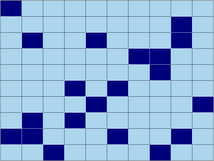

The most common way to assign observations to the training or testing set is to take a simple random sample such that \(Z\%\) of the observations are in the training set and \((100 - Z)\%\) are in the testing set (Figure 10.3 (a)). A common split is 80% training and 20% testing; however, there is no magic number for the best split. The primary consideration for determining a split is the overall size of the sample data and ensuring there are enough observations in the training set to conduct inference and model evaluation. For example, if the data set is small (e.g., 100 observations), perhaps a split of 90% training and 10% testing may be preferred, so that as much data as possible is available for the model building process.
Another common approach is to take a stratified random sample (Figure 10.3 (b)). This may be the preferred approach is there are particular subgroups you want to ensure make up an exact proportion of the observations in the training and testing sets. For example, suppose \(W\%\) of the population is part of a particular subgroup, and we want to ensure exactly \(W\%\) of the observations in the training and testing sets are in that group. In this case, we stratify the data by group, then take \(Z\%\) for training and \((100 - Z)\%\) for testing within each subgroup.
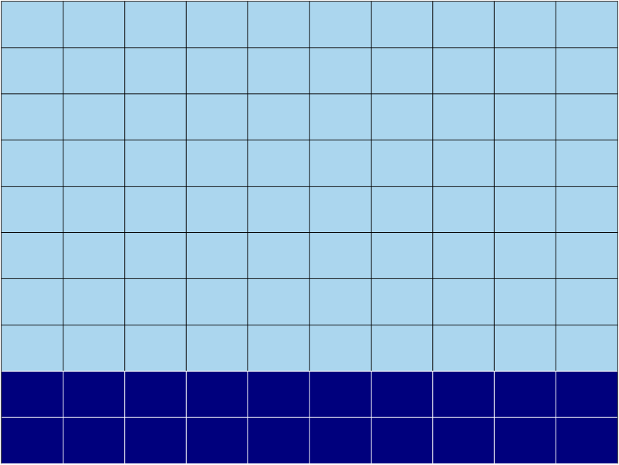
Finally, if time is an important component of the data, another option is to use the most recent time period as the testing set and all previous time periods for the training set (Figure 10.3 (c)). This is especially helpful if the model will be used for predicting future observations (called forecasting).
Once the data have been split into training and testing sets, we use the following workflow.
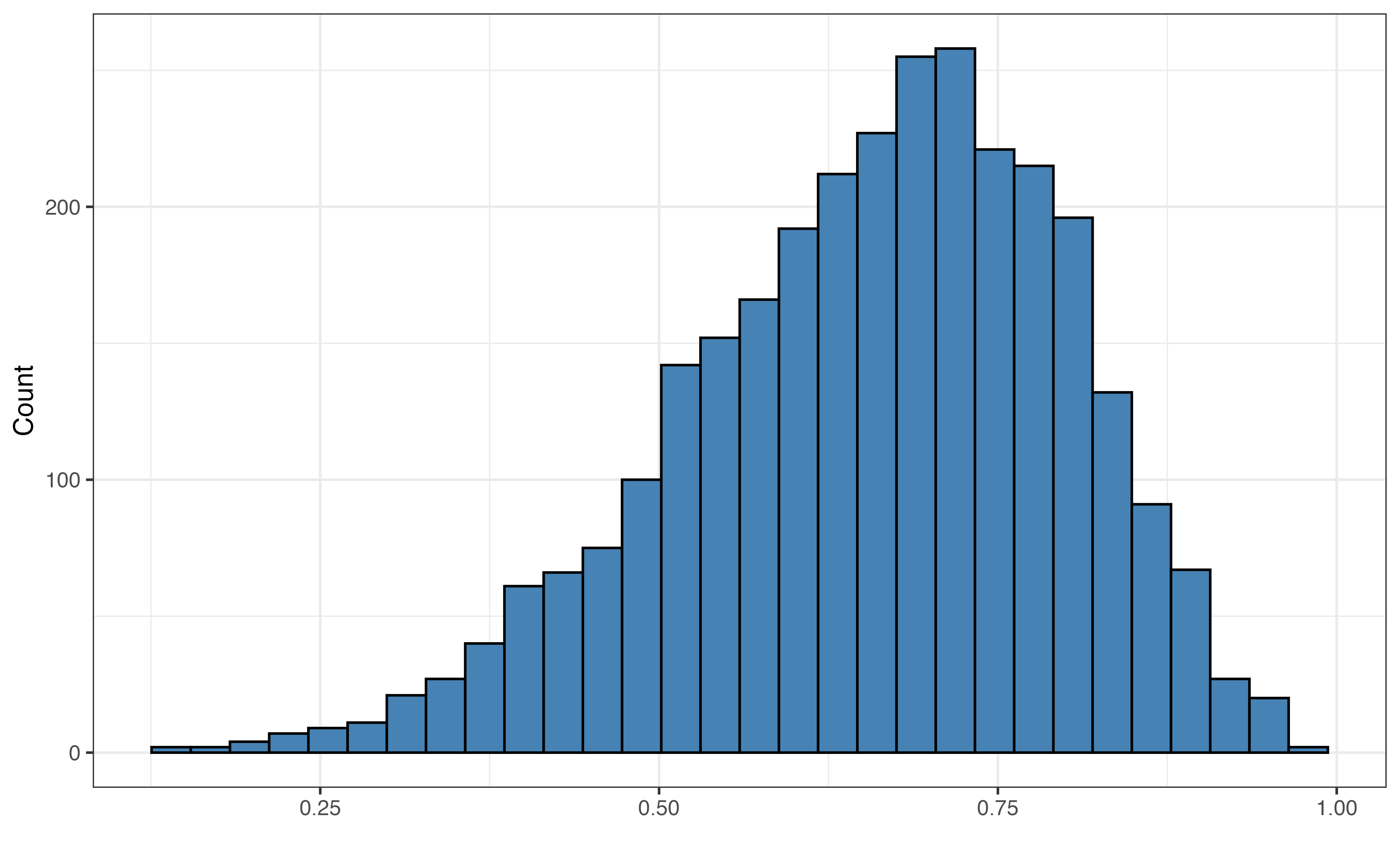
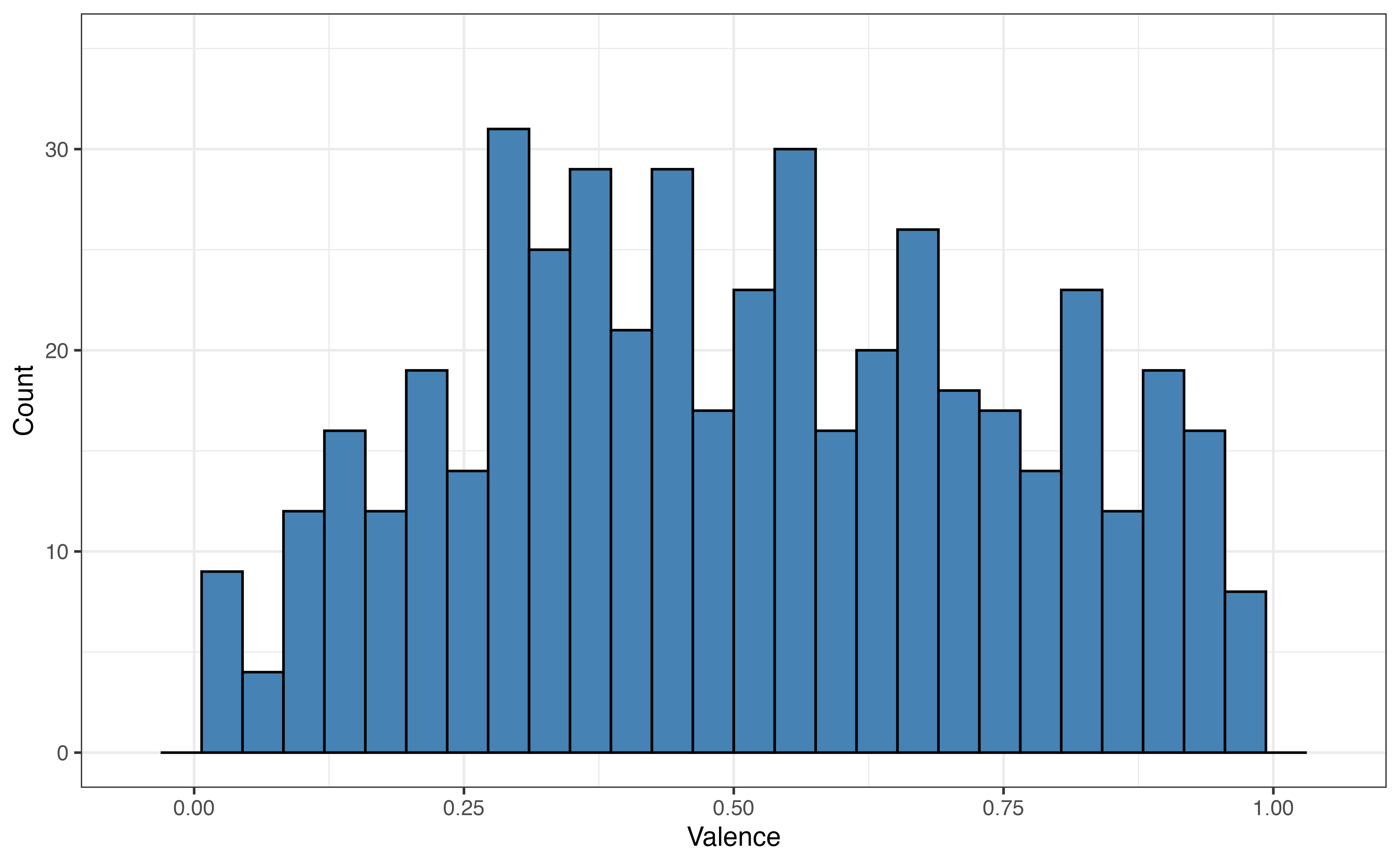
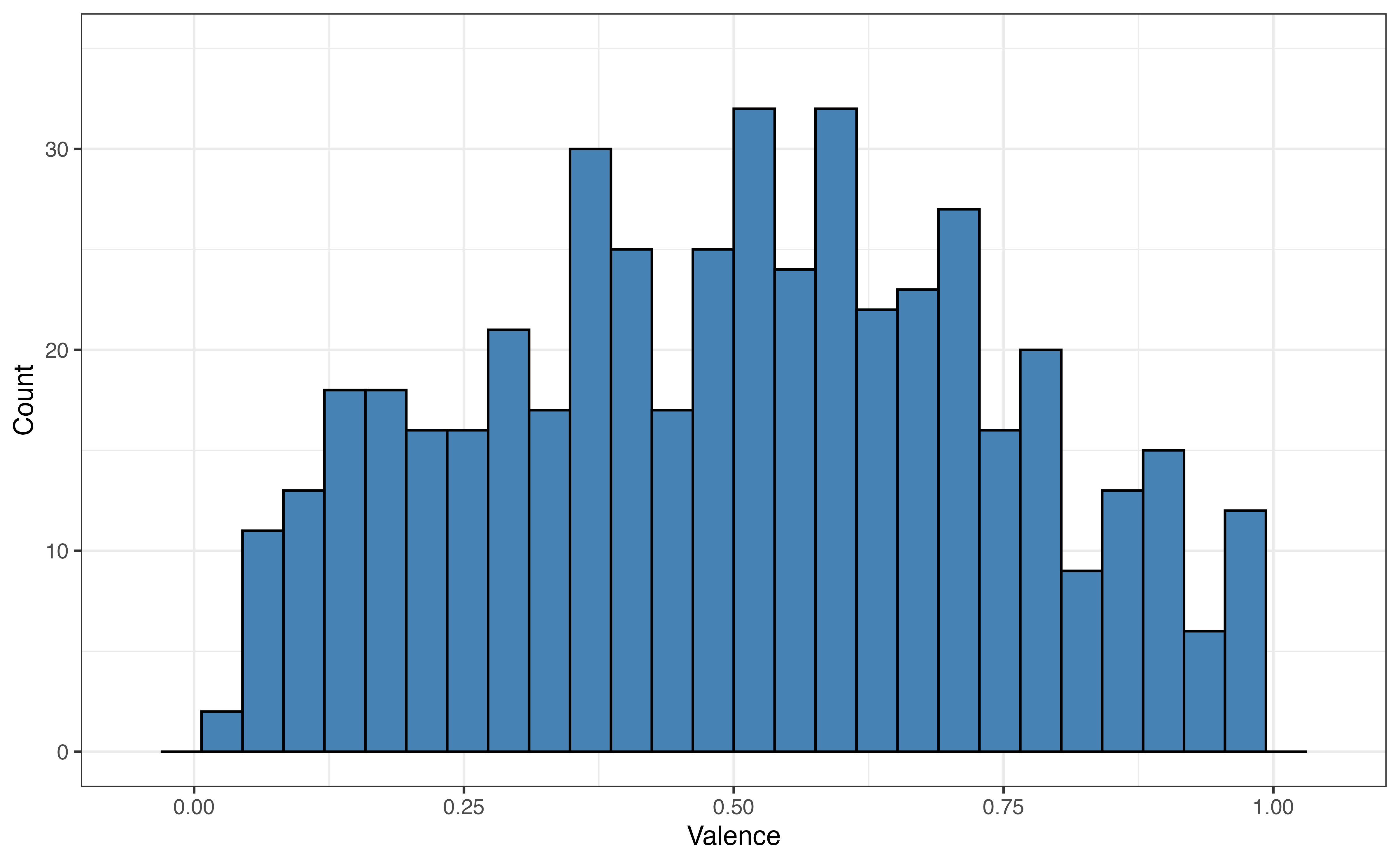
Here we apply this workflow to the Spotify data. First, we split the data into the commonly used 80% training and 20% testing sets. The original sample data has 3000 observations, so the training set has 2400 observations and the testing set has 600 observations. Figure 10.4 shows a comparison of the distribution of valence in the full sample data, training set, and testing set. The distributions have a similar shape and are all centered around 0.5.
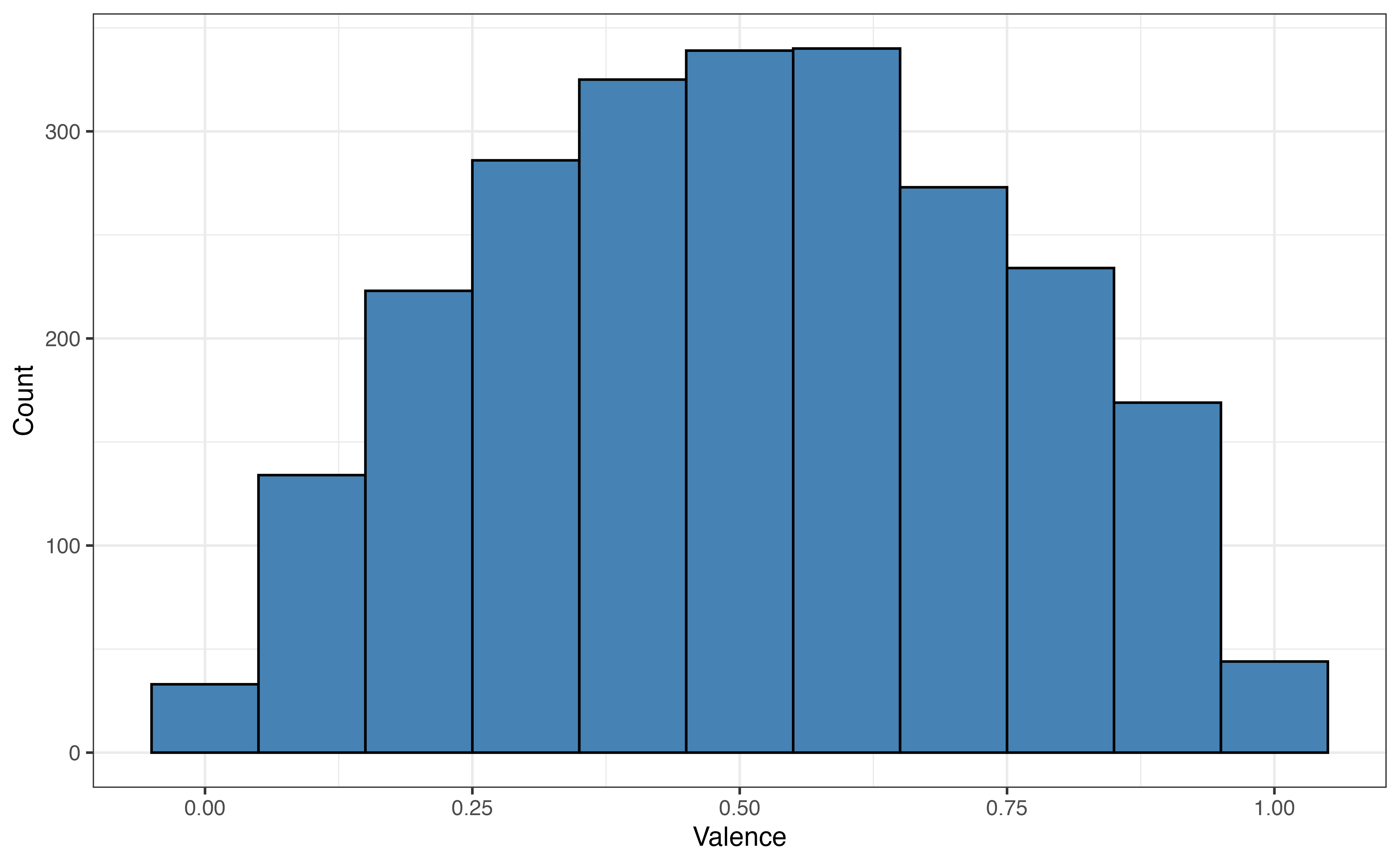
valence in full sample data, training set, and testing set
For now we put the testing set aside and use the training set to build a model. Because the primary analysis objective in Section 10.1 is explanation, we’ll use forward selection with AIC as the selection criteria. Table 10.12 is the model selected by this process.
| term | estimate | std.error | statistic | p.value |
|---|---|---|---|---|
| (Intercept) | -0.424 | 0.051 | -8.28 | 0.000 |
| danceability | 0.629 | 0.033 | 19.25 | 0.000 |
| playlist_genrelatin | 0.215 | 0.014 | 15.12 | 0.000 |
| playlist_genrepop | 0.172 | 0.014 | 12.17 | 0.000 |
| playlist_genrer&b | 0.218 | 0.015 | 14.61 | 0.000 |
| playlist_genrerap | 0.144 | 0.014 | 10.14 | 0.000 |
| playlist_genrerock | 0.230 | 0.016 | 14.65 | 0.000 |
| energy | 0.451 | 0.036 | 12.55 | 0.000 |
| acousticness | 0.107 | 0.022 | 4.94 | 0.000 |
| duration_min | -0.019 | 0.004 | -4.56 | 0.000 |
| loudness | -0.008 | 0.002 | -4.10 | 0.000 |
| tempo | 0.000 | 0.000 | 2.46 | 0.014 |
Next, we check the model conditions and diagnostics from Section 8.5 for the selected model.
Which data set is used to check model conditions - full sample data, training set, testing set?6
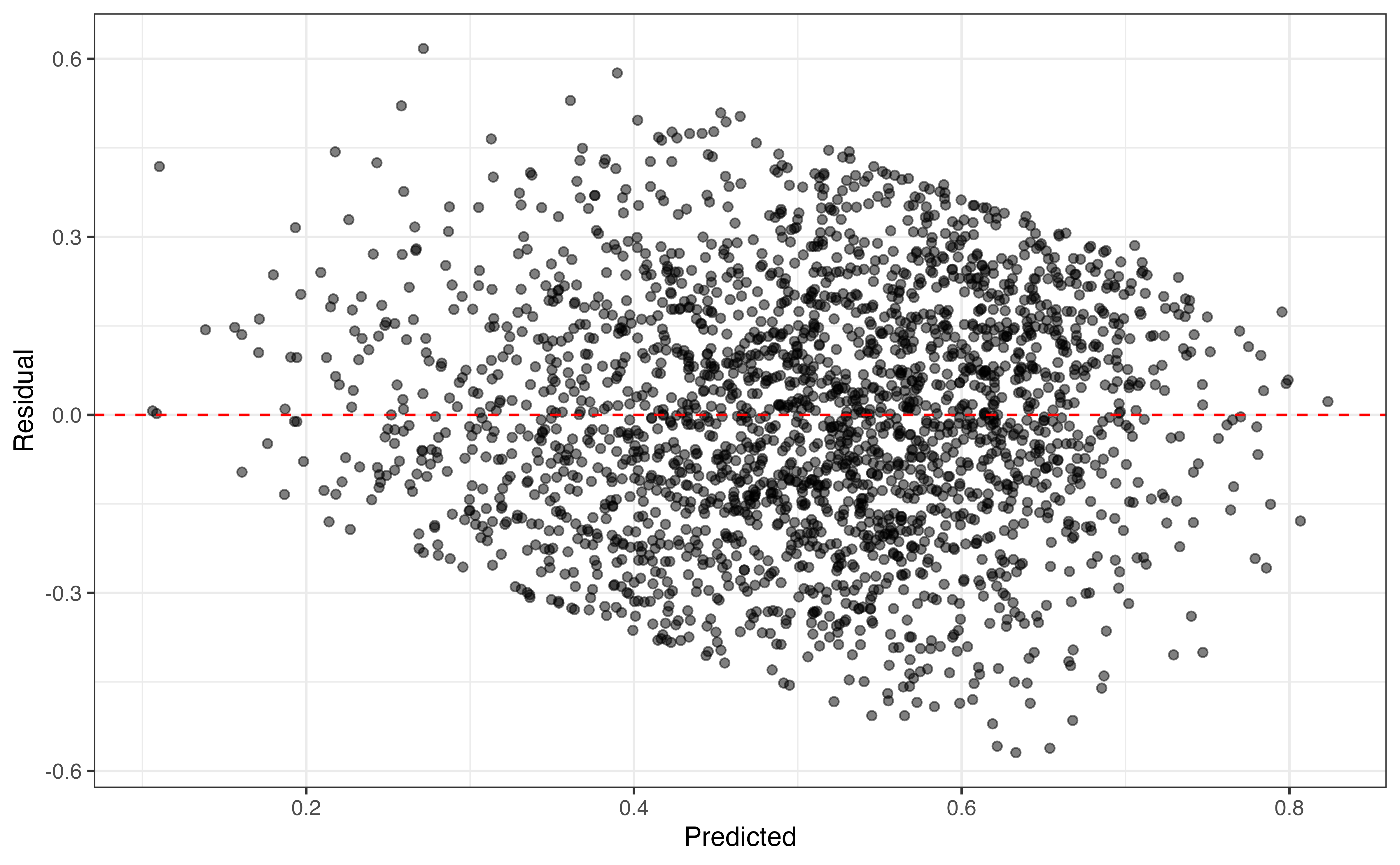
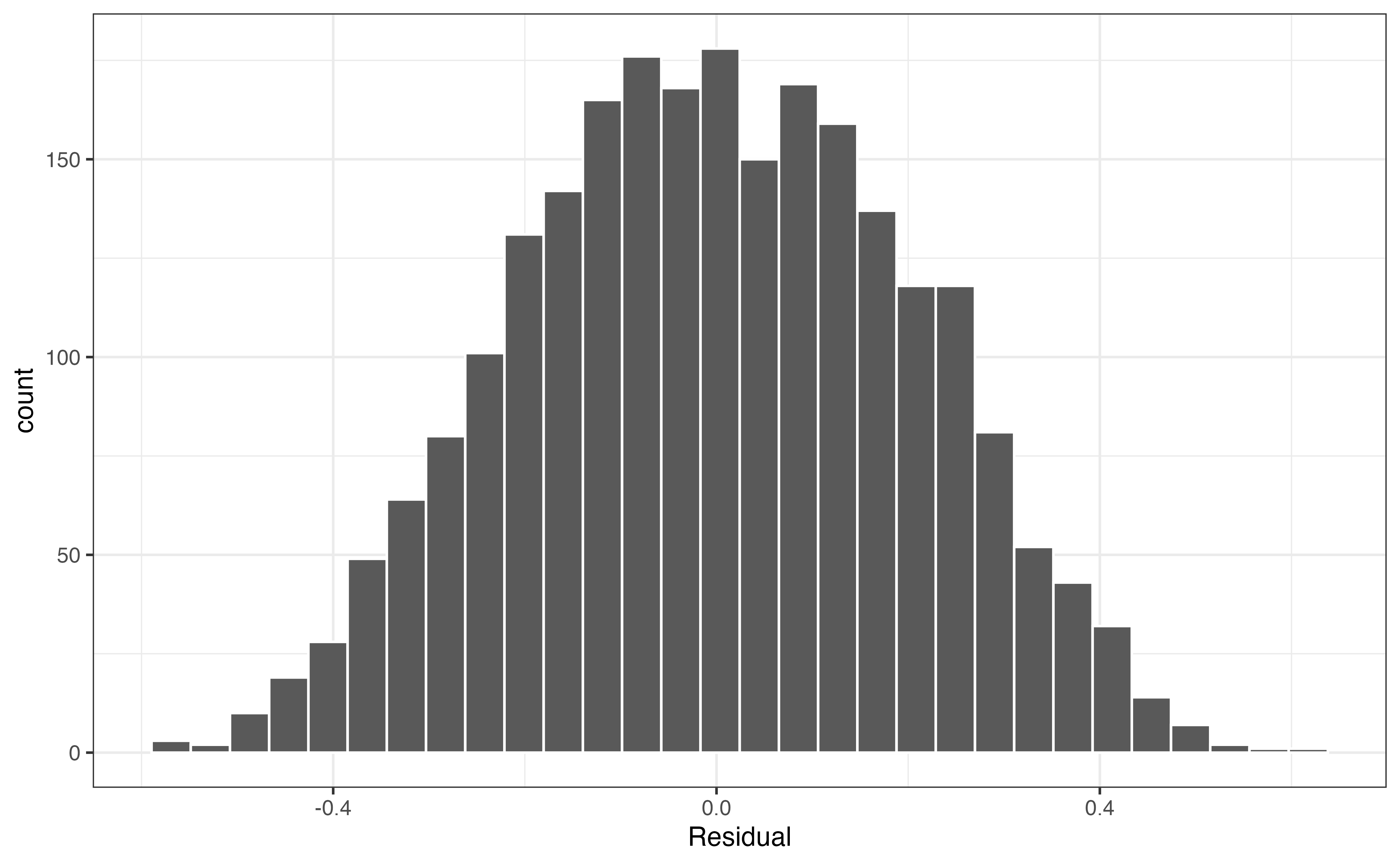
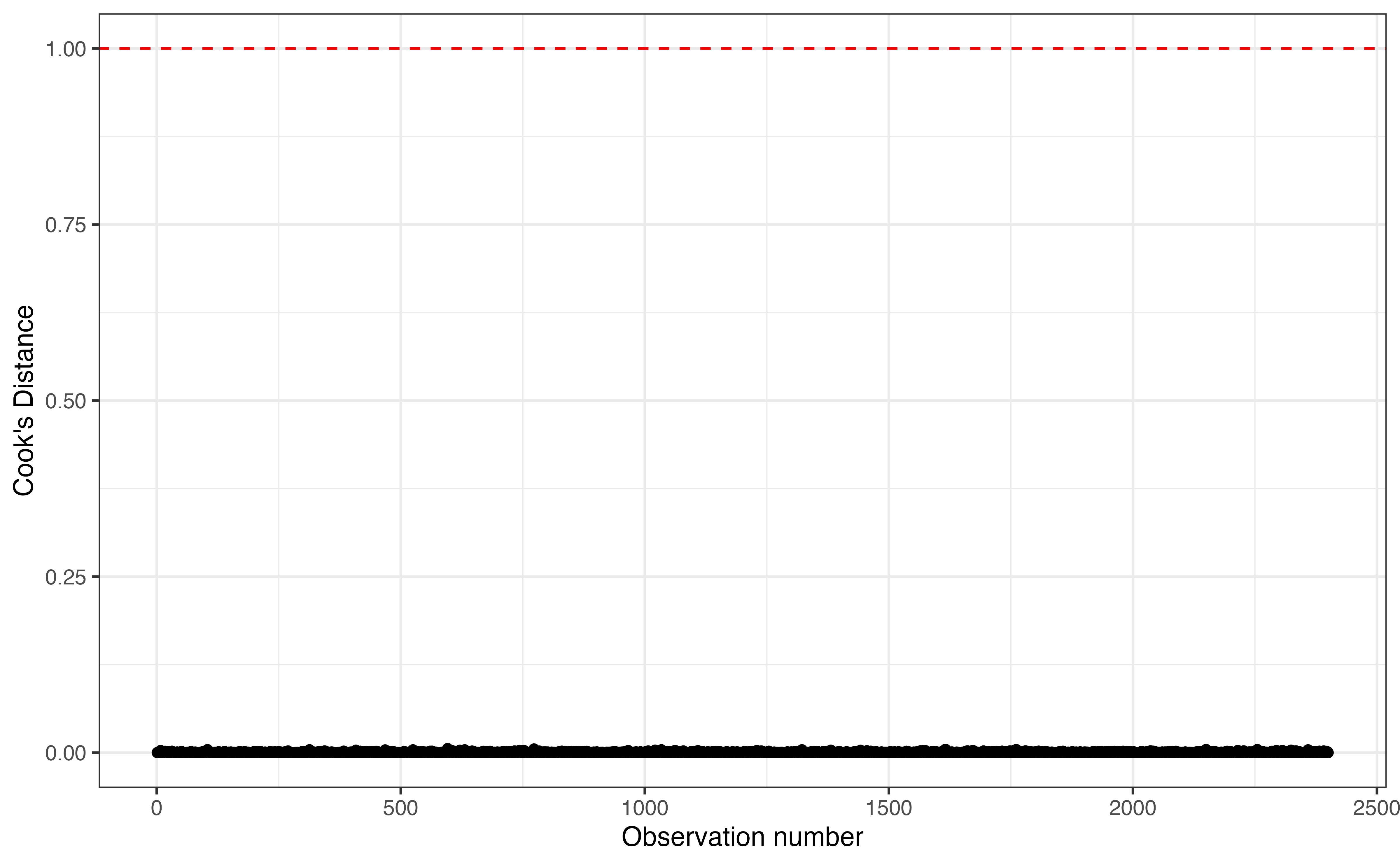
From Figure 10.5, the linearity, equal variance, and normality conditions are satisfied and there are no influential observations based on Cook’s Distance. From the description in Section 10.1, we know that there is only one song for a given artist in the data, so we can reasonably conclude the independence condition is met as well. Table 10.13 shows the RMSE and \(R^2\) on the training set. We prioritize \(R^2\), because the primary analysis objective is explanation.
| R-sq | RMSE |
|---|---|
| 0.257 | 0.204 |
This is a good point in the analysis to consider potential interaction terms, variable transformations, or higher order polynomial terms if there is indication from the exploratory data analysis that such terms would improve model fit. As we try new terms, we use RMSE, \(R^2\), and inferential statistics to evaluate whether to include them in the model. We will proceed with the model in Table 10.12 as the final model for the purposes of this example.
Now that we have selected the final model, we use the model to compute RMSE, \(R^2\), and predictions on the testing set. RMSE and \(R^2\) are then used to evaluate how well the model performs on the testing set.
| Sample, | R-sq | RMSE |
|---|---|---|
| Training | 0.257 | 0.204 |
| Testing | 0.204 | 0.211 |
Table 10.14 shows the values of \(R^2\) and RMSE for the training and testing set. When we fit a model, the goal is to adequately capture the trends in the data without capturing the trends so specifically that the can’t be used on new data. In general, we expect the model performance to be better (lower RMSE, higher \(R^2\)) for the training set, because it was used to fit the model. When we compare these values, we want the results from the testing set to be similar, even if slightly worse, as the training set. When the results are similar, this means that the model can be generalized and reliably applied to new observations in the population. As we implement the model and use it to predict for new observations, we can expect a similar model performance as we have observed in the analysis. In contrast, if the model performs much better on the training set compared to the testing set, then it is indication of overfitting.
The goal when building a model is to capture the trends in the data while still making something that can applied to new data. When a model is overfit, a model will perform very well on the data used to fit it but perform very poorly on any new data. Overfitting generally occurs when there are complex interaction terms between three or more variables or polynomial terms that are cubic or high-order.
Avoid overfitting by preferencing simpler models that adequately capture the trends in the data over those that fit very closely to the training set used to build them.
Remember, model building is like making a suit that can generally fit everyone around a given size, not making a custom-tailored suit that can only fit one person perfectly.
We note in Table 10.14 the model performed better on the training data, but the performance statistics are similar for the training and testing sets. This means that we have not overfit the model to the training set and thus can feel some level of confidence that we understand how the model will perform on new data.
The testing set gives us information about the model performance on new data; however, using a single testing set can make it difficult to know how much the results are impacted by nuances in the data, such as the presence of outliers. Additionally, because the testing set is only used to evaluate the model performance once the model building process is complete, the information about the model’s performance on new data does not inform the final model selection. Having multiple sets for testing during the model selection process would help address these issues.
We could collect more data to make additional testing sets, however, that is often not feasible in practice given time and cost constraints. Therefore, we will use resampling, the process of sampling from the data to generate “new” data sets. We have discussed two resampling methods earlier in the book, bootstrapping and permutation tests in Section 8.3.
Because the goal is to generate multiple testing sets, we will resample in such a way that a different subset of the data is used to build the model and a different subset is used to evaluate the model’s performance on new data in each iteration. We only use the training set for resampling, so we can still reserve the testing set to evaluate the final model. For each iteration of resampling from the training set, the subset of the training set used to build the model is called the analysis set, and the subset of the training set used to evaluate the model is the assessment set. We use these terms from Kuhn and Silge (2022) to distinguish them from the training and testing sets. Figure 10.6 shows the resampling process for \(k\) iterations.
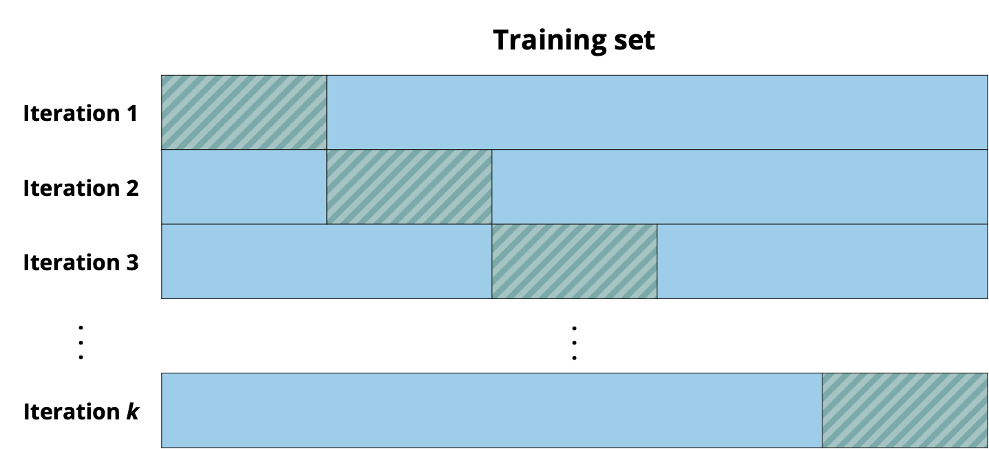
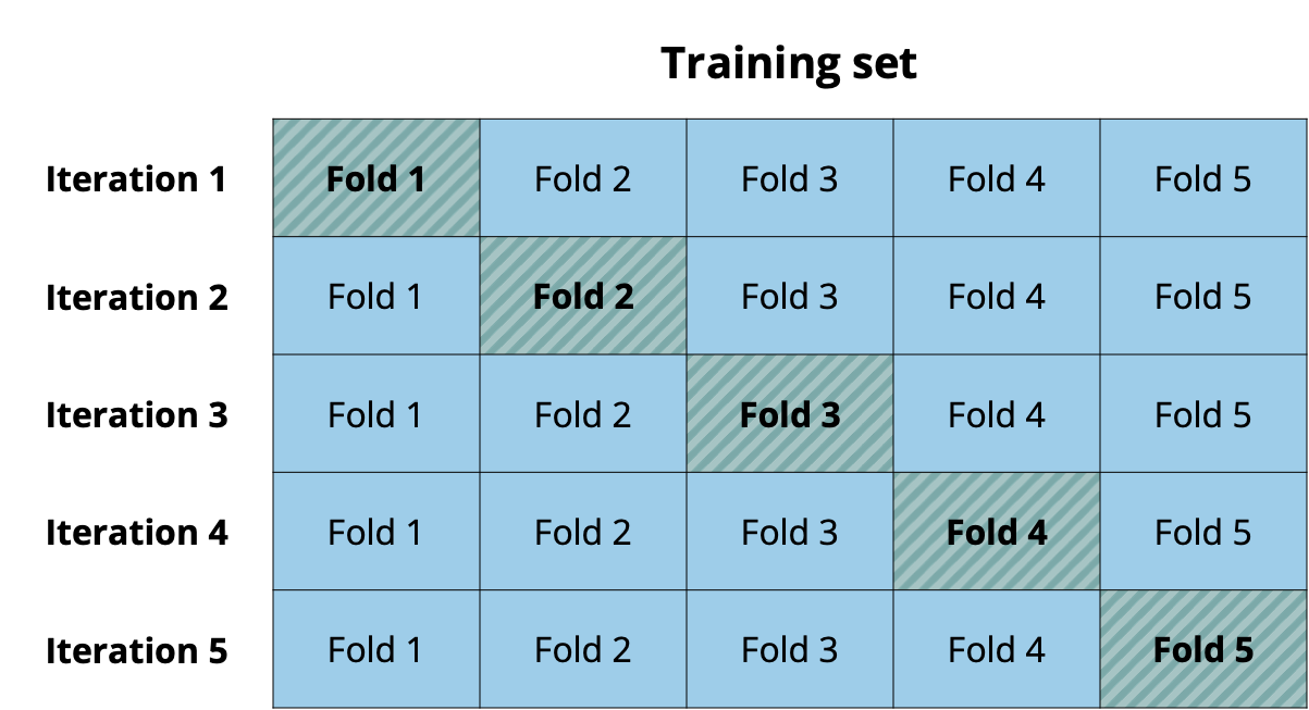
Cross validation (also called k-fold cross validation) is a resampling method that splits the data into \(k\) subsets called folds. Commonly used choices for the number of folds are \(k = 5 \text{ or }10\). In each iteration, \(k - 1\) of the folds make up the analysis set, and the remaining fold makes up the assessment set. At the end of the \(k\) iterations, the model’s overall performance is computed as an average of the performance statistic across all iterations. For example, if we use RMSE to evaluate performance, the model’s overall performance is the average RMSE across the \(k\) iterations. Figure 10.7 illustrates the folds, analysis set, and assessment sets for a 5-fold cross validation.
Because cross validation is only conducted on the training set, a measure of how the model performs on new data (the assessment set at each iteration) can be used to compare potential models and throughout the model building process. As before, the testing set is reserved for providing a final evaluation of the performance of the final model.
Below is the outline of a model building workflow workflow using cross-validation.
While doing cross validation, we are not necessarily concerned with the estimated regression coefficients or their interpretations. In fact, by the end of of Step 3, there will be \(k\) similar (but different!) estimated values for each model coefficient. The purpose of cross validation is to evaluate how well the model predicts for data it has not seen before. It is at the last step of the process that we look closely at the model coefficients, their interpretations, and conclusions about the relationship between the response and predictor variables.
The most commonly used values for \(k\), the number of folds, are 5 and 10. There are few points to consider when choosing \(k\).
Using a smaller value of \(k\)
Use a smaller number of folds there are few observations in the training set. Only one fold is part of the assessment set used to evaluate the model performance at each iteration, so if \(k\) is large, there will be very few observations in the assessment set.
Small values of \(k\) tend to result in more biased estimates of the model performance statistic, for example RMSE. Biased estimates are far from the true (yet unknown!) population statistic, so they can result in an unreliable view of the model performance.
Using a larger value of \(k\)
Cross-validation can be computationally intensive. Larger \(k\) means more resampling and model refitting is required, which can result in long computational times, often for little added value.
Large values of \(k\) result in more variability in the estimated model performance statistic, for example RMSE. This means at each iteration may produce very different estimates of the model performance, resulting in an unreliable evaluation of the model performance.
Choosing \(k = 5\) or \(k = 10\) produces model performance statistics that have little bias and variability, while also reducing the computational intensity. See Chapter 3 of Kuhn and Johnson (2019) and Chapter 5 of James et al. (2021) for more discussion about choosing \(k\).
Here we illustrate the cross validation workflow to fit the full model using all predictors in Section 10.1 to explain variability in the valence of the songs on Spotify. Recall from Section 10.4 the training set has 2400 observations. The training set is split into five folds, with each having 480 observations.
Based on Figure 10.7, which fold(s) make up the analysis set and which make up the assessment set in the first iteration?
For the first iteration of cross validation on the Spotify training set, how many observations will be in the analysis set? How many in the assessment set?7
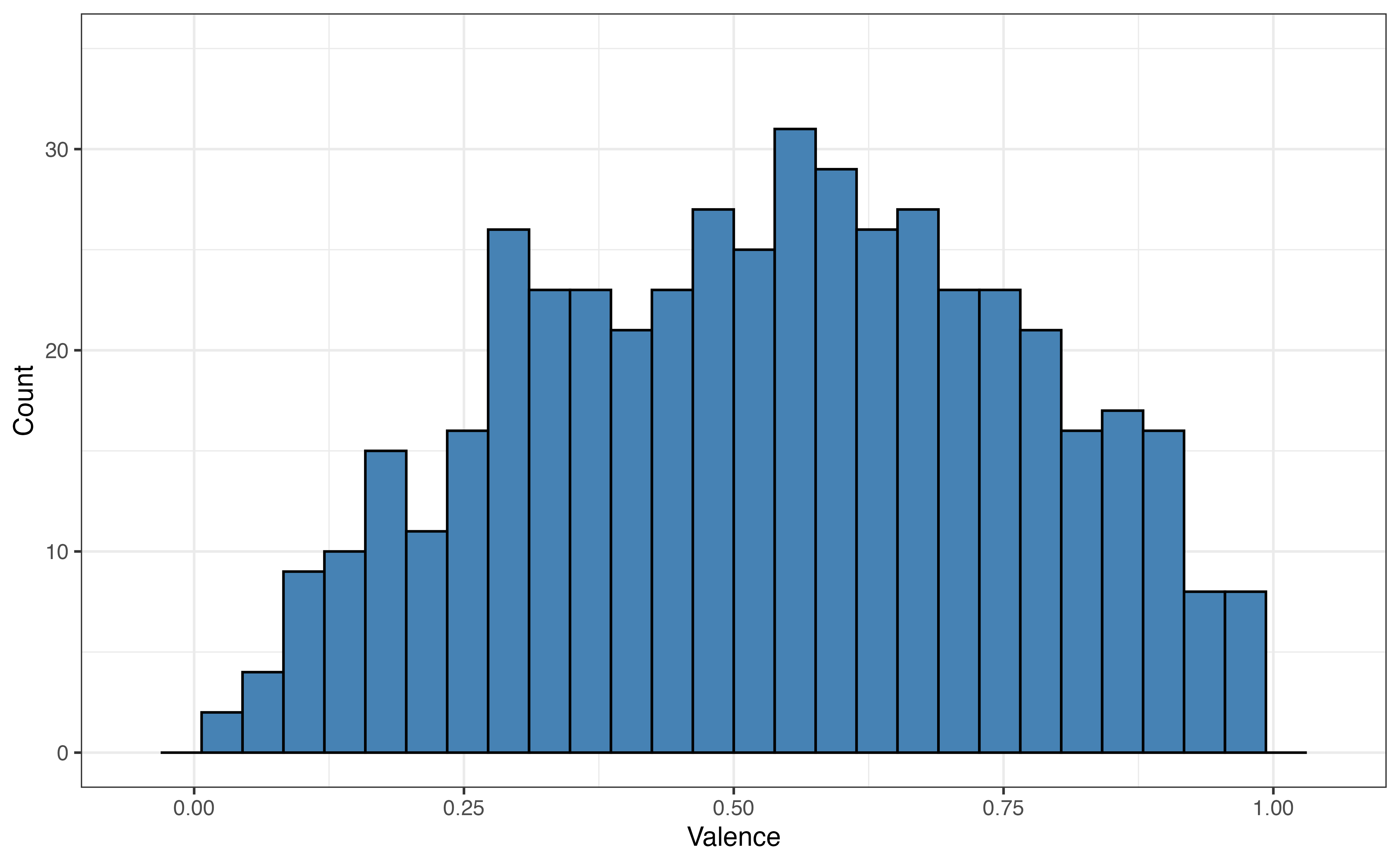
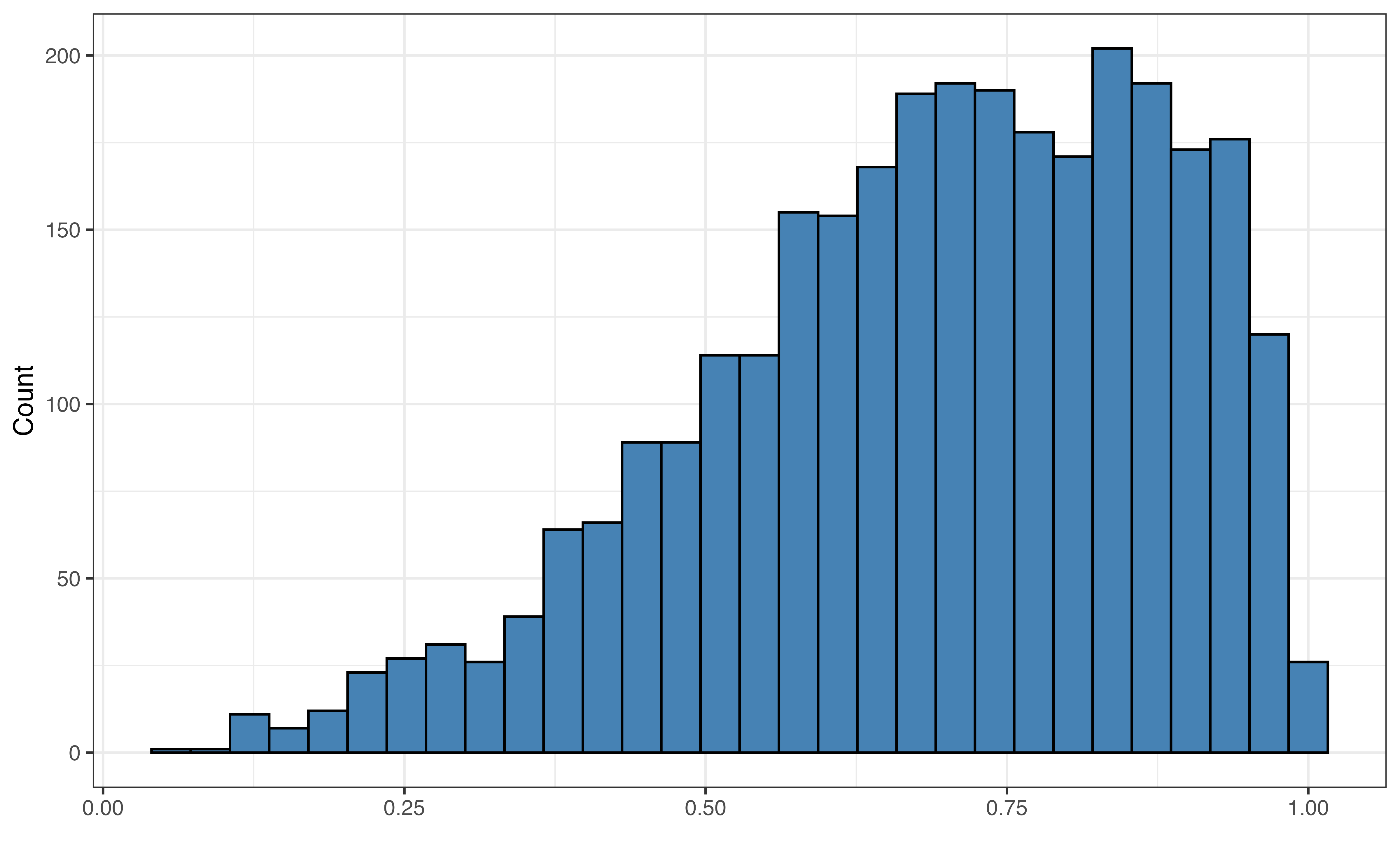
valence for 5 folds
Figure 10.8 shows the distribution of the the response variable valence for each fold. As we expect from random sampling, the distribution of valence is very similar across the folds.
Next, we fit the full model using the analysis set in each of the five iterations. Recall from Figure 10.7, that in each iteration the analysis set consists of four folds and one fold is held out as the assessment set. For example, from Figure 10.7, in Iteration 5, Folds 1 - 4 are the analysis set and Fold 5 is the assessment set.
| Term | Iteration 1 | Iteration 2 | Iteration 3 | Iteration 4 | Iteration 5 |
|---|---|---|---|---|---|
| (Intercept) | -0.432 | -0.408 | -0.484 | -0.407 | -0.420 |
| playlist_genrelatin | 0.216 | 0.229 | 0.199 | 0.216 | 0.221 |
| playlist_genrepop | 0.167 | 0.178 | 0.151 | 0.181 | 0.187 |
| playlist_genrer&b | 0.215 | 0.222 | 0.205 | 0.224 | 0.228 |
| playlist_genrerap | 0.150 | 0.146 | 0.130 | 0.153 | 0.146 |
| playlist_genrerock | 0.227 | 0.226 | 0.220 | 0.245 | 0.236 |
| danceability | 0.656 | 0.596 | 0.675 | 0.608 | 0.630 |
| energy | 0.415 | 0.435 | 0.475 | 0.456 | 0.465 |
| loudness | -0.007 | -0.008 | -0.009 | -0.008 | -0.008 |
| modeMinor | -0.009 | 0.002 | -0.002 | -0.007 | 0.001 |
| acousticness | 0.108 | 0.102 | 0.127 | 0.112 | 0.090 |
| liveness | 0.055 | 0.020 | -0.008 | 0.018 | 0.042 |
| tempo | 0.001 | 0.000 | 0.000 | 0.000 | 0.000 |
| duration_min | -0.018 | -0.016 | -0.013 | -0.021 | -0.025 |
Table 10.15 shows the estimated model coefficients from each iteration of cross validation. The coefficients are similar but not exactly the same across each iteration, because the analysis set used to fit the models at each iteration are similar but not exactly the same. The coefficients are displayed here to provide a glimpse into the process, but in practice we are not concerned with the estimates of the model coefficients at this point in the analysis. Instead, we are most concerned with the model performance.
| Fold | R2 | RMSE |
|---|---|---|
| Fold1 | 0.202 | 0.256 |
| Fold2 | 0.212 | 0.262 |
| Fold3 | 0.209 | 0.226 |
| Fold4 | 0.207 | 0.245 |
| Fold5 | 0.201 | 0.233 |
Table 10.16 shows \(R^2\) and RMSE computed from the assessment set in each iteration, measuring the model’s performance on new data. As with the model coefficients, there is some variability in these statistics, but they show a similar model fit. In practice, we are most interested in the average values across all folds. The average \(R^2\) is 0.244 and the average RMSE is 0.206.
In practice, these values are most helpful when comparing multiple candidate models during the model selection process. Let’s compare the results of cross-validation for the full model to the results of cross-validation for the model selected by forward stepwise selection in Table 10.8. Note that we will use the same folds for both models, so that we are comparing the models’ performances on the same analysis and assessment sets.
| Model | RMSE | R-sq |
|---|---|---|
| Full model | 0.206 | 0.244 |
| Forward selection | 0.206 | 0.246 |
From Table 10.17, the results from 5-fold cross validation are very similar for the full model and the model selected by forward selection. Thus, there is no clear preferred model based on these model performance results. At this point, we would rely on our judgment as data scientists and the original analysis objective to choose between these models. Given the aim to select the simplest model, we may choose the model selected by forward selection over the full model.
The glance() function in the broom package (Robinson, Hayes, and Couch 2025) is used to compute Adjusted \(R^2\), AIC, and BIC. It also includes other model fit statistics, such as log-likelihood used to compute AIC and BIC.
spotify_model <- lm(valence ~ danceability + mode + liveness,
                    data = spotify)

glance(spotify_model) |>
  select(adj.r.squared, AIC, BIC)
# A tibble: 1 × 3
adj.r.squared AIC BIC
<dbl> <dbl> <dbl>
1 0.0951 -424. -394.The Root Mean Square Error is obtained by first computing the predicted values, then using rmse() from the yardstick package (Kuhn, Vaughan, and Hvitfeldt 2025). The code below uses augment() to compute the predicted values.
spotify_model_aug <- augment(spotify_model)

rmse(spotify_model_aug, truth = valence, estimate = .fitted)
# A tibble: 1 × 3
.metric .estimator .estimate
<chr> <chr> <dbl>
1 rmse standard 0.225Forward and backward selection are conducted using the step() in the stats base R package. For both selection methods, we define the intercept-only model (called the null_model) and the model with all candidate predictors (called the full_model). The code below shows how to specify each model for the Spotify data analysis using various features of a song to predict valence.
null_model <- lm(valence ~ 1, data = spotify)
full_model <- lm(valence ~  playlist_genre + danceability + energy +
                   loudness + mode +  acousticness + liveness +
                   tempo + duration_min,
                         data = spotify)
Next is the code to conduct forward selection. The final model chosen by forward selection is saved as forward_model.
forward_model <- step(null_model,
                      scope = formula(full_model),
                      direction = "forward",
                      trace = 0,
                      k = 2)
The argument trace = 0 will suppress all the intermediate results from the stepwise process. Use trace = 1 to display output from each step of the forward selection.
The step function uses AIC as the selection criteria by default, as shown by k = 2. Use the argument k = log(nrow(my_data)) to use BIC as the model selection criteria. For example, we use k = log(nrow(spotify)) to use BIC as the selection criteria for this analysis.
The code for backward selection is similar to the code for forward selection. Primary differences are how the scope are defined and the direction.
backward_selection <- step(full_model,
                           scope = list(lower = formula(null_model),
                                        upper = formula(full_model)),
                           direction = "backward",
                           trace = 0,
                           k = 2)
The step function can only use AIC or BIC as the model selection criteria. An alternative stepwise selection function is regsubsets() in the leaps R package (Miller 2024). It can use a variety of model selection criteria, such as Adjusted \(R^2\), and residual sum of squares (SSR, which is proportional to RMSE).
Data can be split into training and testing sets using functions from the resample package (Frick et al. 2025).
The function initial_split() is used to randomly assign observations to the training and testing set. The argument prop = defines the proportion of observations that are assigned to the training set. Because this is a random process, use set.seed() for reproducibility to ensure the same assignment each time the code is run.
The code below randomly assigns 80% of the observations to the training set and 20% of the observations to the testing set.
set.seed(12345)

spotify_split <- initial_split(spotify, prop = 0.8)
spotify_split
<Training/Testing/Total>
<2400/600/3000>The data in the training and testing sets can be extracted using the functions training() and testing() respectively. We save the sets under the object names spotify_train and spotify_test and will call these objects in subsequent steps of the analysis.
We conduct cross validation using functions from the resample and workflows (Vaughan and Couch 2025) packages. The folds are defined using the vfold_cv() in the resamples package. It uses the argument v = to define the number of folds. Below is the code to create the folds for 5-fold cross validation. Note that we use spotify_train, the training set.
set.seed(12345)
folds <- vfold_cv(spotify_train, v = 5)
folds
# 5-fold cross-validation
# A tibble: 5 × 2
splits id
<list> <chr>
1 <split [1920/480]> Fold1
2 <split [1920/480]> Fold2
3 <split [1920/480]> Fold3
4 <split [1920/480]> Fold4
5 <split [1920/480]> Fold5The output indicates that for each fold, there are 1920 observations in the analysis set and 480 observations in the assessment set. If we wish to examine the data in each fold more closely (for example, as in Figure 10.8), we are able to extract the data contained in each fold. Below is code to extract the data in the analysis and assessment sets for Fold 1.
fold1_analysis <- folds$splits[[1]] |> analysis()

fold1_assessment <- folds$splits[[1]] |> assessment()
Once the folds are defined, we use the workflow(), add_model(), and add_formula() functions from the workflows package to specify the model that will be fit in each iteration of cross validation. The code below defines the workflow for fitting the full model from the Spotify data.
spotify_workflow.
Next, we use fit_resamples() from the rsamples package and collect_metrics() from the tune package (Kuhn 2025) to fit the specified model to each of the 5 analysis sets and obtain the performance metrics.
spotify_workflow. Save the models fit in cross validation as spotify_cv.
fold.
# A tibble: 2 × 6
  .metric .estimator  mean     n std_err .config
  <chr>   <chr>      <dbl> <int>   <dbl> <chr>
1 rmse    standard   0.207     5 0.00104 pre0_mod0_post0
2 rsq     standard   0.237     5 0.0113  pre0_mod0_post0
The default for collect_metrics() is to produce the average performance statistics, as indicated by the argument summarize = TRUE . We can use summarize = FALSE to print the performance statistics for each iteration.
collect_metrics(spotify_cv, summarize = FALSE)# A tibble: 10 × 5
id .metric .estimator .estimate .config
<chr> <chr> <chr> <dbl> <chr>
1 Fold1 rmse standard 0.207 pre0_mod0_post0
2 Fold1 rsq standard 0.230 pre0_mod0_post0
3 Fold2 rmse standard 0.206 pre0_mod0_post0
4 Fold2 rsq standard 0.274 pre0_mod0_post0
5 Fold3 rmse standard 0.210 pre0_mod0_post0
6 Fold3 rsq standard 0.204 pre0_mod0_post0
# ℹ 4 more rowsThe full code workflow for 5-fold cross validation is below.
set.seed(12345)

# define the folds
folds <- vfold_cv(spotify_train, v = 5)

# specify the model
spotify_workflow <- workflow() |>
  add_model(linear_reg()) |>
  add_formula(valence ~ playlist_genre + danceability + energy +
                loudness + mode + acousticness + liveness +
                tempo + duration_min)

# fit the model to the analysis set in each fold
spotify_cv <- spotify_workflow |>
  fit_resamples(resamples = folds)

# obtain performance statistics for each iteration
collect_metrics(spotify_cv, summarize = TRUE)
There are many ways to customize cross validation, including the sampling process used to define the folds and the performance statistics computed at each iteration. We point interested readers to Chapter 10 of Kuhn and Silge (2022) for more details on customizing cross validation in R.
In this chapter, we reviewed and introduced statistics for measuring model fit and predictive performance. We discussed how to determine which statistics to prioritize based on the primary modeling objective and introduced stepwise methods for model selection. We introduced a model selection workflow using training and testing sets, and expanded this with cross validation. Lastly, we described how to implement a complete model selection workflow and showed how to do so in R.
Here we introduced the basics of cross-validation, but there are many iterations of cross validation, including Leave One Out Cross Validation (LOOCV) and Monte Carlo cross validation. There are also extensions of the training and testing set, such as validation set that can be used alongside the training set in the model building process. We point readers to Chapters 10 and 11 of Kuhn and Silge (2022) and Chapter 3 of Kuhn and Johnson (2019) as starting points for more advanced discussion of these topics.
So far, we have discussed linear regression models for quantitative response variables. In Chapter 11, we look beyond quantitative response variables and introduce logistic regression, models for categorical response variables.
Answers may vary. Danceability and Energy appear to be the most strongly associated with valence based the bivariate graphs. Both show a positive relationship - more danceable songs tend to be more positive and more high energy songs to be more positive.↩︎
We generally select the model with lower RMSE, because it means the model is producing more accurate predictions, on average.↩︎
Based on (Kass and Raftery 1995)↩︎
Based on (Burnham and Anderson 2002, pg. 70)↩︎
We would choose the model with the single predictor danceability based on AIC, because it has the smaller value. The same is true for BIC. Based on the guidelines in Table 10.3, AIC gives weak evidence and BIC gives very strong evidence in favor of this model.↩︎
The training set. The training set is used for the entire model building process.↩︎
Based on Figure 10.7, Folds 2 - 5 are the analysis set and Fold 1 is the assessment set in Iteration 1. There will be 1920 observations in the analysis set (4 folds) and 480 observations in the assessment set (1 fold).↩︎