| Variable | Mean | SD | Min | Q1 | Median (Q2) | Q3 | Max | Missing |
|---|---|---|---|---|---|---|---|---|
| life_exp | 71.6 | 8.1 | 51.6 | 65.4 | 72.8 | 78.0 | 84.1 | 0 |
| income_inequality | 19.8 | 9.7 | 5.4 | 11.5 | 18.1 | 28.3 | 44.2 | 0 |
1 Regression in the data science workflow
Learning goals
- Define regression analysis and how it is used to answer questions about real-world phenomena
- Describe the data science workflow
- Define reproducibility and how it is implemented in the data science workflow
1.1 Regression analysis
We use data to gain insights and knowledge about real-world phenomena. Often, there is a population we are interested in studying (e.g., all adults in the United States), but we do not have access to data on the full population. Or we want to make predictions for what is expected to happen in the population in the future. In either case, we analyze data about a sample (subset) drawn from the population to gain insights or make predictions about the population. The sample is made of the observations in the data obtained in the collect stage of Figure 1.3.
One way this is done, in general, is through statistical models. Statistical models are a broad array of mathematical models that are used to describe how data are generated in the population (also called data generating models). This text will primarily focus on a class of statistical models called regression analysis.
Population: Entire group being studied
Sample: Subset of the population that is used in the analysis
Statistical model: Mathematical models used to describe how data are generated in a population
1.1.1 What is regression analysis?
Regression analysis (also called regression models) is a set of statistical models that describe multivariable relationships, the relationships between two or more variables. In particular, they describe the relationship between a response variable and one or more predictor variables. The response variable (also called outcome or dependent variable) is the outcome of interest. In other words, it is the variable about which we wish to understand variability or predict. The predictor variables (also called explanatory variables or independent variables) are the variables used to explain variability or predict the response variable. We denote the response variables \(Y\) and the predictor variables as \(X_1, X_2, \ldots, X_p\), where \(p\) is the number of predictors.
Regression analysis: Set of statistical models to describe multivariable relationships between a response and one or more predictor variables
Response variable: Variable whose variability we wish to understand or we wish to predict
Predictor variable(s): Variable(s) used to explain variability in the response or to predict new values of the response variable
In regression analysis, we assume the values of the response variable be generated by the following process
\[ Y = \text{Model} + \text{Error} \tag{1.1}\]
More specifically, the model is a function of the predictor variables, \(\text{Model} = f(X_1, X_2, \ldots, X_p)\) . We input some values of the predictor variables and the output is \(f(X_1, X_2, \ldots, X_p)\). The Error, then, is the difference between the observed value \(Y\) and the output from \(f(X_1, X_2, \ldots, X_p)\). Much of regression is choosing the \(\text{Model}\) and using the \(\text{Error}\) to evaluate the model’s performance and how well it explains the relationships in the data.
There are two types of regression models that differ on how they define \(f(X_1, X_2, \ldots, X_p)\). Breiman (2001) referred to these as the “two cultures” of statistical modeling.
In parametric regression models, we assume the model function takes a specific form and then use techniques to estimate the parameters of the model. For example, we may assume the model takes the form
\[ f(X_1, X_2, \ldots, X_p) = \beta_0 + \beta_1X_1 + \beta_2X_2 + \dots + \beta_pX_p \tag{1.2}\]
where \(\beta_0, \beta_1, \beta_2, \ldots, \beta_p\) are the model coefficients. Thus, the full form of the model from Equation 1.1 is
\[ \begin{aligned} &Y = f(X_1, X_2, \ldots, X_p) + \epsilon \\[10pt] \Rightarrow &Y = \beta_0 + \beta_1X_1 + \beta_2X_2 + \dots + \beta_pX_p + \epsilon \end{aligned} \tag{1.3}\]
where \(\epsilon\) is the error.
In parametric regression, we use regression methods to fit the model, find estimated values for these model coefficients. We then input these estimated coefficients into Equation 1.2 to produce predicted values of the response variable, denoted \(\hat{Y}\).
\[ \hat{Y} = \hat{\beta}_0 + \hat{\beta}_1X_1 + \hat{\beta}_2X_2 + \dots + \hat{\beta}_pX_p \]
When we fit models using parametric methods, we make inherent assumptions about the underlying form of the relationships in the data. In Chapter 6, we show ways to check a set of model conditions to evaluate whether these assumptions are actually true in the data. One advantage to parametric models is that we can use them to interpret the relationship between the response and predictor variables. In Chapter 4 and Chapter 7, we will talk extensively about how we might interpret the estimated coefficients, and how for example, we can use this equation to predict values of life expectancy. For now, the goal is to see that when using parametric methods, we derive a mathematical equation of the relationship between the response variable and predictor variables then estimate the coefficients in that equation.
The vast majority of this book focuses on parametric models, specifically linear regression (models for quantitative response variables) and logistic regression (models for categorical response variables).
The second type of regression model is non-parametric regression models. These models differ from parametric models in that there is no assumed structure of the function between the response and predictor variables. The function \(f(X_1, X_2, \ldots, X_p)\) is defined by finding a way to closely model the trend in the sample data without fitting it so closely that it couldn’t apply to new data. The advantage to this approach is that we do not impose an assumed structure on the relationship between the response and predictor variables. The primary disadvantage, however, is that these models are often uninterpretable, making it difficult to describe the relationships in the data.
Parametric regression: Methods in which the model structure is predefined and the data are used to estimate coefficients of the model
Non-parametric regression: Methods in which there is no predefined structure for the model, and the model is defined by getting close (to a point) to the observations
Fit a model: Use data to estimate a model
1.1.2 Why fit a regression model?
In general, there are two primary purposes for regression analysis: inference and prediction. Inference is the process of drawing conclusion and insights from the model. Prediction is the process of computing the expected value of the response variable based on values of the predictor variable(s).
Both tasks are often performed in a single analysis. It is generally beneficial to be able to use a model to generate both predictions and insights from the data. The analysis questions from plan stage of the data science workflow (Figure 1.3) are used to determine the primary purpose of an analysis. As we will see throughout the book, many analysis decisions are made based on whether the analysis is focused on inference or prediction (or both).
Inference: Process of drawing conclusions and insights from a model
Prediction: Process of computing the expected value of the response variable based on value(s) of the predictor variable(s)
Here, we are interested in models that are intperpretable and are useful for gaining insights about the data. Even as evaluate models with prediction as the primary objective, we still take the interpretability into account. Therefore, we will often balance predictive accuracy with ease of interpretation. This is often important for models that are used in research, as the goal is to use data to understand a particular phenomena. In other contexts, such as industry for example, the importance of predictive accuracy may far exceed the that of interpretability. In this case, non-parametric models, such as those commonly used in machine learning, may be preferred over regression methods. We will discuss a set of non-parametric models in ?sec-cecision-trees and refer readers to Introduction to Statistical Learning (James et al. 2021) for a more in-depth introduction to non-parametric models.
1.1.3 Example: Country’s life expectancy
We apply what we’ve discussed about regression models thus far to an example motivated by Zarulli et al. (2021), who studied the relationship between life expectancy and a country’s healthcare system. Life expectancy is how long an individual is expected to live on the day they are born based on factors about their surrounding environment. There are large differences in life expectancy around the world, so it is important to understand the factors that impact life expectancy in order to help improve outcomes for individuals in countries with lower life expectancy.
In this section, we will use data from Zarulli et al. (2021) to examine the relationship between life expectancy, education, and income inequality. The data were originally obtained by researchers from the Human Development Database (https://hdr.undp.org/data-center) and the World Health Organization (https://apps.who.int/nha/database).
The data set is available in life-expectancy.csv. It contains information about life expectancy, health-care related factors, and other societal factors for 140 countries. We will use the following variables in this section. The definitions are from the respective original data sources.
life_exp: The average number of years that a newborn could expect to live, if he or she were to pass through life exposed to the sex- and age-specific death rates prevailing at the time of his or her birth, for a specific year, in a given country, territory, or geographic area. (from the World Health Organization)income_inequality: Measure of the deviation of the distribution of income among individuals or households within a country from a perfectly equal distribution. A value of 0 represents absolute equality, a value of 100 absolute inequality (Gini coefficient). (from the Human Development Database)education: Indicator of whether a country’s education index is above (High) or below (Low) the median index for the 140 countries in the data set.- Education index: Average of mean years of schooling (of adults) and expected years of school (of children), both expressed as an index obtained by scaling wit the corresponding maxima. (from the Human Development Database)
See Zarulli et al. (2021) for a full codebook.
Figure 1.1 shows the distributions and Table 1.1 shows the summary statistics for life_expectancy and income_inequality. These are used to better understand the data, a process called exploratory data analysis (EDA). EDA is introduced more fully in Chapter 3.
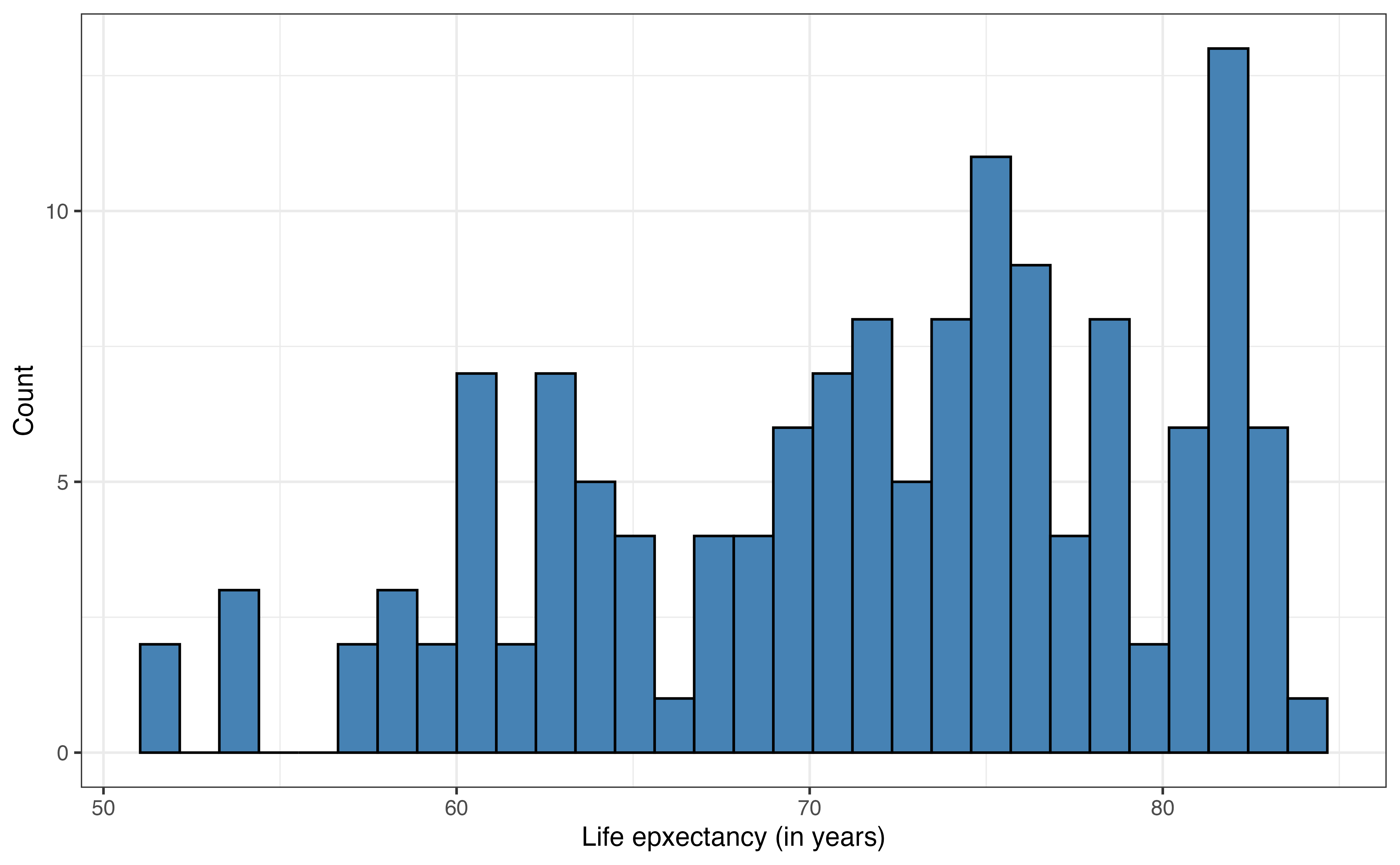
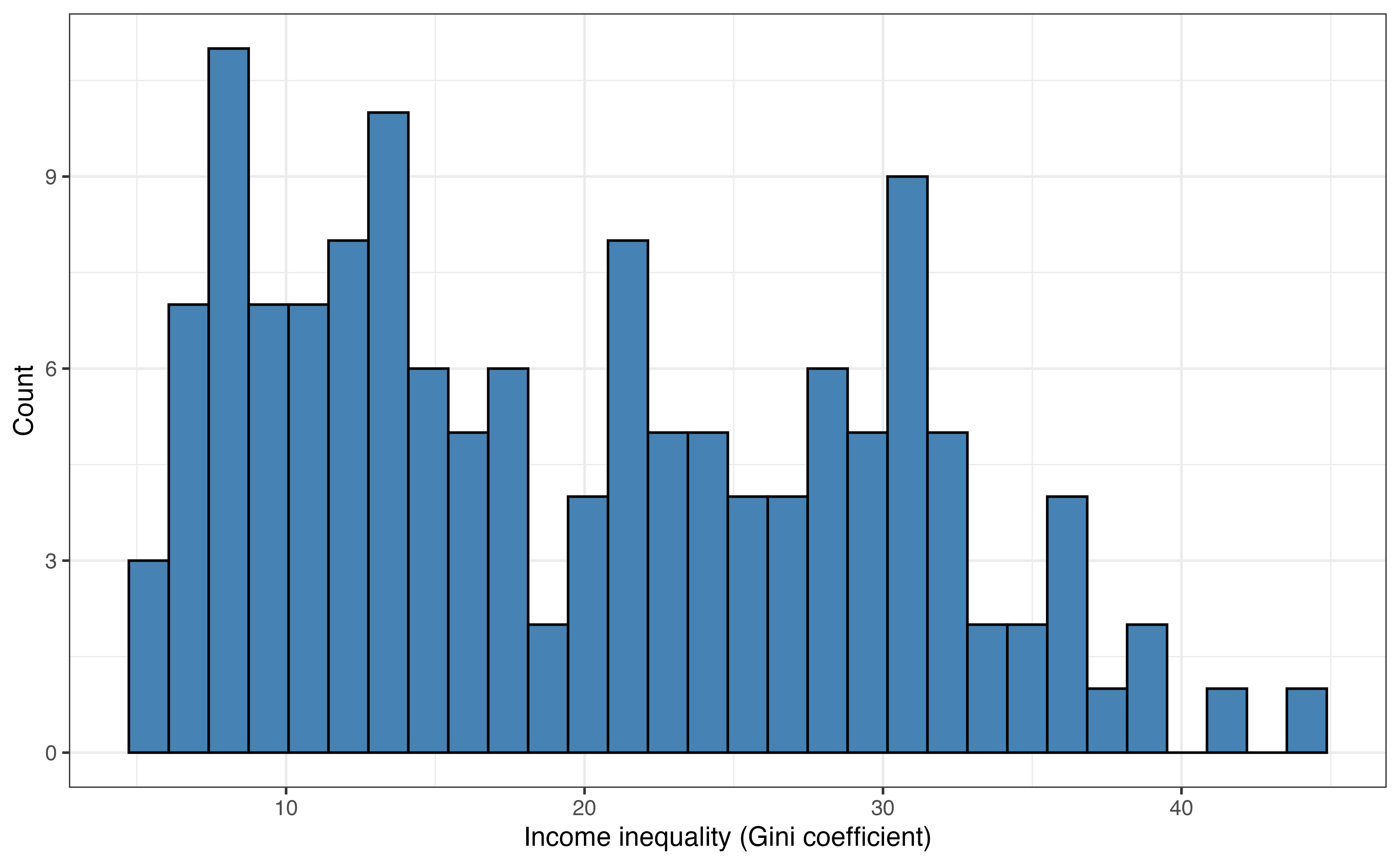
What do you observe about the distributions of life_exp and income_inequality based on Figure 1.1 and Table 1.1?1
We know the distribution of education based on its definition. Fifty percent of the observations are categorized as Low and 50% are categorized as High.
Suppose we wish to fit a regression model to predict a country’s life expectancy using income inequality and education. In parametric regression, we can specify the form of the model as
\[ \begin{aligned} \text{life\_exp} &= f(\text{income\_inequality},\text{education}) + \epsilon \\[10pt] & = \beta_0 + \beta_1~\text{income\_inequality} + \beta_2~\text{education} + \epsilon \end{aligned} \tag{1.4}\]
In Section 1.1.2, we introduced the two primary purposes of regression analysis, prediction and inference.
- What is an example a prediction question that can be answered from Equation 1.4?
- What is an example of an inference question that can be answered from Equation 1.4?2
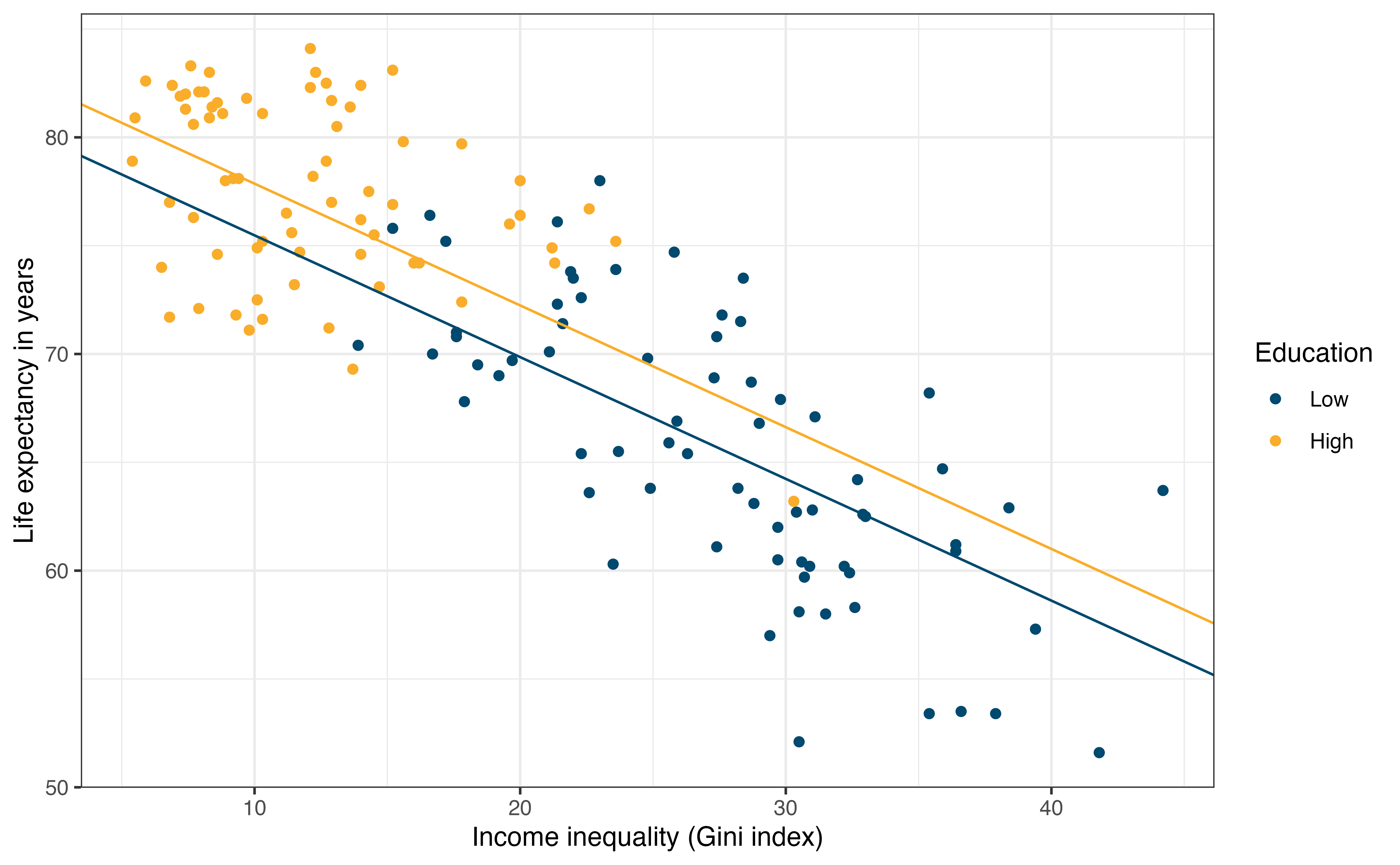
We use the data to fit the model and find estimates for \(\beta_0, \beta_1, \text{ and }\beta_2\). Equation 1.5 is the equation of the estimated model, and Figure 1.2 is a visual representation of this model. We discuss the process of choosing the model form, estimating the coefficients, and interpreting the model beginning in Chapter 4.
\[ \widehat{\text{life\_exp}} = 81.096 -0.562 \times \text{income\_inequality} + 2.386 \times \text{education} \tag{1.5}\]
1.2 Regression in a data science workflow
Regression is typically one step in a larger data science workflow. In this section, we will zoom out so we can see where regression fits in the context of this workflow.
1.2.1 Data science approach
Data science is a relatively new and rapidly evolving discipline, and there is no single definition of what data science is and how it compares to related disciplines. This book approaches regression through the lens of data science, so let’s take a moment to explore how others have defined data science and use it to describe what it means to use take a “data science approach” to regression.
In the 1962 paper The Future of Data Analysis, statistician John Tukey describes the field of data analysis, which many argue is actually a description of what we call data science today. He says data analysis includes
“procedures for analyzing data, techniques for interpreting the results of such procedures, ways of planning the gathering of data to make its analysis easier, more precise or more accurate, and all the machinery and results of (mathematical) statistics which apply to analyzing data.” (Tukey 1962, 2)
He later on goes to argue that data analysis is, in fact, a science, because it contains the three characteristics of a science
- intellectual content
- organization into an understandable form,
- reliance upon the test of experience as the ultimate standard of validity. (Tukey 1962, 5)
The way we think about and work with data has changed dramatically since Tukey’s 1962 definition of “data analysis”. Today, data are ubiquitous and have become integrated into every day life, and very large data sets (called “big data”) have become increasingly common. Additionally, the “machinery” that Tukey refers to has become much more sophisticated and widely accessible, vastly increasing the data analysis capabilities available to researchers, industry professionals, and learners alike.
Given these differences in today’s data landscape, let’s look at some more recent definitions of data science.
Wikipedia defines data science as
“an interdisciplinary academic field that uses statistics, scientific computing, scientific methods, processing, scientific visualization, algorithms and systems to extract or extrapolate knowledge from potentially noisy, structured, or unstructured data.” (Wikipedia contributors 2025)
In Modern Data Science with R, Baumer, Kaplan, and Horton (2017) define data science as “science of extracting meaningful information from data”. In R for Data Science, Wickham, Çetinkaya-Rundel, and Grolemund (2023) say it is “an exciting discipline that allows you to transform raw data into understanding, insight, and knowledge.” In Data Science: A First Introduction, Timbers, Campbell, and Lee (2022) define data science as the “process of generating insight from data through reproducible and auditable processes”. In Telling Stories with Data, Alexander (2023) concludes that data science is
“the process of developing and applying a principled, tested, reproducible, end-to-end workflow that focuses on quantitative measures in and of themselves, and as a foundation to explore questions”
Lastly, Alby (2023) emphasizes the domain knowledge in their definition of data science in the book Data Science in Practice,
“Data science is currently still a consolidating application area of artificial intelligence in which interdisciplinary knowledge from statistics, computer science, and expert knowledge from other disciplines are converged to further develop methods for unlocking data patterns in these fields.” (pg. 17)
These definitions tend to emphasize different aspects of data science; however, there are common themes across all of them. Taking these definitions into account, as we introduce regression analysis using a “data science approach”, we are conducting regression such that the following hold:
- We apply knowledge, skills, and tools from statistics and computer science.
- We use domain knowledge to interpret results and glean useful insights from data.
- We conduct analysis using a reproducible workflow.
Pillars (1) and (2) are illustrated throughout the book as we walk through case study examples in each chapter. Pillar (3) is best demonstrated as these methods are put into practice, so we introduce the concept o f a reproducible workflow in Section 1.2.3, discuss tools for conducting reproducible analyses in Section 2.7, and practice implementing it as part of the assignments in the supplemental materials.
Data science approach to regression
We conduct regression analysis such that the following hold:
- We apply knowledge, skills, and tools from statistics and computer science.
- We use domain knowledge to interpret results and glean useful insights from data.
- We conduct analysis using a reproducible workflow.
1.2.2 Data science workflow
The focus of this book, regression analysis, is one part of a much larger data science workflow. It is important to understand what happens before and after regression modeling, because each step in the workflow informs the others.
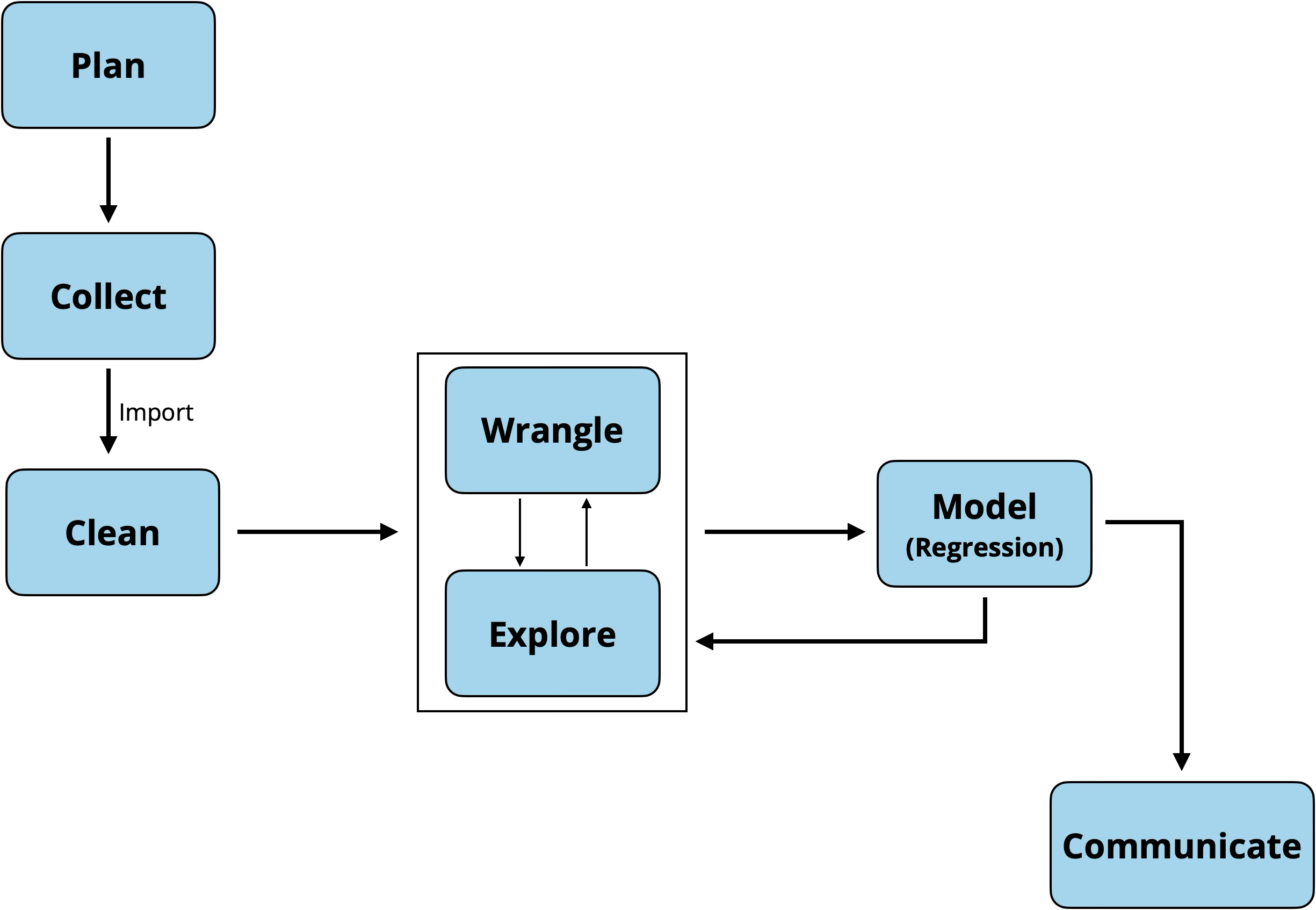
Figure 1.3 is the general data science workflow. As illustrated in Figure 1.3, the process begins before any data analysis. The first step is plan, which starts with clearly defining the analysis (or research) question. In practice, this step is often done in collaboration with subject matter experts (e.g., business partners or research collaborators). The analysis question informs decisions made at each step of the workflow, so it is important to take the time to clearly define it at this step. Additionally, given the vast amounts of data available, having a clear analysis question helps us focus and navigate through what could otherwise be an overwhelming amount of data.
Once the analysis question has been defined, the next step is collect. This is the point in which we collect the data that will be analyzed to answer the analysis question. Data scientists are often data consumers, individuals who work with data that has already been collected (Gebru et al. 2021), so in practice, this stage is focused on obtaining the correct sample data from an existing data set or data base. It is important for the data scientist understand the data provenance, a record of the origins of a data set along with any processing or changes it has undergone since its original creation. Additionally, it is important to review the codebook, documentation of the variables in the data set and their definitions. As we learn more about the data and what the variables measure, we may need to refine the analysis question posed in the previous step to one that can be feasibly answered from the available data. Having an understanding about the contents and history of the data also provides important context as we interpret analysis results.4
Now it’s time to start working with the data. We import it into the statistical software, then begin to clean (or preprocess) the data. This is the point we ensure the data has imported correctly and begin to check for potential errors or missingness in the data. We talk more about this step in Section 3.3.
Next, we wrangle and explore the data, often called exploratory data analysis. This is the point in which we really begin to understand the observations in the data, distributions of the variables in the data, and relationships between variables. We begin to think about the regression modeling, so we may create new variables from existing ones, start to consider how to handle outliers or deal with missing observations. We talk about this step extensively in Chapter 3.
- Data consumers: individuals who work with data that have already been collected (Gebru et al. 2021)
- Data provenance: Record of a dataset’s origin and history of changes
- Codebook: Documentation of variables in a data set
After we have explored the data it is time to model the data, the primary topic of this text. This is where we apply statistical methods to more rigorously describe relationships between variables and glean insights from the data to answer the analysis questions posed in the first step. Note from Figure 1.3 that we often iterate through modeling, exploring, and wrangling, as the modeling may uncover areas in which we need to consider variable transformations (Chapter 9) or consider new relationships in the data.
Once we have finalized the model and drawn conclusions, it’s time to communicate the results. This is a very important step in the workflow, because as Wickham (2014) put it, “the end product of an analysis is not a model: it is rhetoric”. We often conduct data science to inform decisions, such as informing business decisions or to share new knowledge through innovative research results. Therefore, it is important that we accurately and effectively communicate the results of the work to collaborators, stakeholders, and sometimes a general audience. Throughout the book, we will discuss how to communicate interpretations and conclusions from the regression model, along with various nuances that can make our communication more or less effective.
Because the goal of this book is to introduce regression analysis methods, the “model” part of the data science workflow will be given out-sized attention, compared to the time it often takes in practice. We will illustrate the other parts of the workflow throughout, because they are important for fully understanding and using the regression analysis results, and to remind us that regression analysis is one part of a larger data science workflow.
1.2.3 Reproducibility
The third pillar of the data science approach introduced in Section 1.2.1 is using a reproducible workflow. Alexander (2023) defined a reproducible workflow as one “which can be exactly redone, given all the materials used…The minimum expectation is that another person is independently able to use your code, data, and environment to get your results, including figures and tables.” Using this definition as the baseline, we will discuss the following components of a reproducible workflow:
- Data
- Code and analysis reports
- Version control
- Organization
- Environment
Reproducibility is infused throughout the data science workflow in Figure 1.3, from the initial plan through communicating results using reproducible tools. The components of reproducibility are introduced separately to help organize our thinking, but they are greatly intertwined in practice. For example, it is difficult to talk about best practices for coding without taking into account the data.
1.2.3.1 Data
The first component of a reproducible workflow is clear documentation for the data. We introduced the notion of data sheets from Gebru et al. (2021) to document data provenance and a codebook to document the variables in the data set. The data sheet provides background for the data that is useful context as we interpret results. The codebook is documentation of the individual variables, so we are clear about what is measured as we conduct the analysis. In general, a codebook should include the following details for each column in the data set:
- Column name
- Data type (e.g., quantitative, categorical, date, identifier)
- Precise definition of the variable
- Possible range of values or categories
- Units (if applicable)
Sometimes codebooks have incomplete information. If information about the data provenance or about individual variables are missing, work with collaborators who are knowledgeable about the data collection process if available, or use exploratory data analysis (Chapter 3) to fill in as much missing information as possible.
1.2.3.2 Code and analysis reports
We will use the statistical software R for the analyses in the book. The code and analyses will be written in one of two file types when using R: scripts (.R) and Quarto documents (.qmd). In general, we use scripts for processes that produce output but not analyses (e.g., creating data sets and writing functions). In contrast, we use Quarto documents for more complete analyses in which there is code, output, and narrative for the process and interpretation of results. This book focuses on complete analyses, so Quarto documents should be used. Quarto documents are more formally introduced in Section 2.7.
Part of making code reproducible is making it readable to other users (including future you). In this text, we will do this, in part, by utilizing the tidyverse, a specific R syntax that utilizes human-readable names. The tidyverse is introduced in Section 2.3. Additionally, we use narrative in Quarto documents or comments in scripts to describe what a set of code is doing. The goal is not to explain every line of code, but to give general ideas about what analysis task is being done in a set of code and the motivation for doing it. Comments and narrative can also be helpful to explain parts of code that may not be immediately obvious to another reader (or future you) (Alexander 2023).
We can further improve the readability of code through the choice of naming convention for variables and functions and how the code is formatted. See Chapter 4 of R for Data Science (Wickham, Çetinkaya-Rundel, and Grolemund 2023) for further reading on code style to improve readability.
1.2.3.3 Version control
Version control is a “system that records changes to a file or set of files over time so that you can recall specific versions later.” (Chacon and Straub 2014) The ability to systematically track changes to a file helps make work more reproducible and aids in collaboration. Instead of saving new versions of a file each time we update it (i.e., my-analysis.qmd, my-analysis-v2.qmd, my-analysis-final.qmd, my-analysis-final-updated.qmd), we practice version control by documenting the changes made to a single file and making it easier to see the history of changes. It is also useful for debugging code, as version control allows makes it easier to go back to a version of the file before the coding issues occurred.
Git is a software used for version control. It is installed on a computer or virtual machine and configured to use with the analysis software. Throughout an analysis, we write commit messages, short and informative messages that describe the changes that have been made to a document (e.g., Added model interpretation). These changes are committed (saved)and tracked in git. It is similar to the track changes feature in a word processor with the addition of messages that briefly describe the changes at each iteration.
GitHub (https://github.com) and GitLab (https://gitlab.com) are two online platforms for storing git-based projects. They serve as a nice space to backup git-based projects along as a centralized platform for collaboration on git-based projects. They are similar to cloud storage platforms such as Dropbox or Google Drive, with additional functionality specific to git.
The assignments in the supplemental materials are designed to for regular version control throughout. The book Happy Git and GitHub for the useR (Bryan 2020) is a great reference for the technical details about installing and using git and GitHub with R.
Version control: Process of systematically tracking changes to a file
git: Software used for version control
GitHub/ GitLab: online platforms for storing git-based projects
Commit messages: Short and informative messages to describing a change
Commit: Save and store changes in git
1.2.3.4 Organization
It is good practice to keep all files associated with a given analysis within a single folder to make it easy for you and others to navigate. These folders are called projects in RStudio and workspaces in Positron, the data analysis software platforms made by Posit.
An advantage of housing all files for an analysis within a single folder is that files can referenced using relative paths (e.g., data/mydata.csv instead of User/id1234/my-project/data/my-data.csv). Relative paths are important for reproducibility and collaboration, because the path names still work when the project is opened on different computers.
Other considerations for organization are the file structure and naming conventions. There are many ways to organize and name files within a single analysis folder, so it is important to choose a file structure and naming conventions that are most easily understood by you and your collaborators. At a minimum, files should be named in such a way that can be easily read by both humans and the computer. Chapter 7 of R with Data Science (Wickham 2014) and Chapter 3 of Telling Stories with Data (Alexander 2023) provide examples and tips on file structure and naming.
1.2.3.5 Environment
The last, and perhaps most overlooked, component of reproducibility is the computing environment in which the analysis was done. In the context of analyses using R, the environment means the version of the R packages (collections of functions) used for the analysis. Software changes over time, so documenting the environment is key for long-term reproducibility.
There are a few ways to do this in R. A rigorous approach is using the renv R package (Ushey and Wickham 2025) which stores the R packages in the project directory (Wickham, Çetinkaya-Rundel, and Grolemund 2023). Another option is to run the function sessionInfo() and save the results in the project directory. This function will print give information about the R version, details about the computer, packages, and their versions.
1.3 As much art as it is science
“All sciences have much of art in their makeup.” Tukey (1962)
Doing regression analysis (and data science in general) requires a blend of art and science. Good regression analysis needs both rigorous theory-based methods and the judgment (the “artistry”) of the data scientist as they make decisions throughout the analysis process. In the same way a chef relies on their knowledge to make decisions about how much seasoning to add to dish, a data scientist relies on their understanding of statistical methods to make decisions as they prepare, explore, model, and interpret data.
Tukey (1962) argues that data analysis (or regression analysis in our case) is not just an application of statistical theory with the sole objective to “optimize” but rather requires a “heavy emphasis on judgement.” He goes on further to say that to analyze data well, “it must be a matter of judgment, and ‘theory’ whether statistical or non-statistical, will have to guide, not command” [pp. 10]. This judgment is not arbitrary, but come from three sources (summarized from Tukey (1962)):
- judgment based on domain knowledge
- judgment based on knowledge statistical methods
- judgment based on experience from analyzing a variety of data
Throughout the book, we will demonstrate how judgment is used to make decisions in the analysis, particularly as the regression models become more complex in later chapters. As much as we will highlight parts of the decision-making process, using judgment and doing the “art” of regression analysis can’t be learned by merely reading a textbook. It is a skill that is developed after consistent practice working with data. As the world becomes increasingly driven by artificial intelligence, it is this ability to infuse the “art” along with the science that will continue to make human data scientists indispensable.
1.4 Summary
In this chapter, we introduced the data science workflow and the how regression analysis fits within that workflow. We defined reproducibility and the components to take into account when developing a reproducible workflow. We introduced regression analysis, why we fit regression models (inference and prediction), and the role of judgment (“art”) in regression analysis (and data science in general).
The next chapter Chapter 2 is a review (or short introduction) to using the tidyverse for data wrangling, visualization, and writing reproducible reports in Quarto.
Example answers: Have the countries have life expectancy of 72.8 years or higher. There are a few countries with low life expectancy less than 55 years. There appear to be two subgroups of countries in regard to income inequality; those with income inequality between 5 and 15 and those between 20 and 30. There are two countries with high income inequality over 40.↩︎
Example prediction question: What is the life expectancy for a country with high education and no income inequality?
Example inference question: How does a country’s life expectancy change as income inequality increases?↩︎This workflow is inspired by the data science workflows in Wickham, Çetinkaya-Rundel, and Grolemund (2023) and Timbers, Campbell, and Lee (2022).↩︎
Sometimes the data scientist is part of the data collection process, thus making them one of the data creators (Gebru et al. 2021), in addition to being a data consumer. As a data creator, it is imperative to provide detailed documentation about the data, so that data consumers have the necessary information to make informed decisions about the data. See Gebru et al. (2021) for more on data documentation.↩︎