6 Model conditions and diagnostics

6.1 Learning outcomes

Describe how the model conditions (LINE) correspond to the assumptions for linear regression
Use the data to check model conditions
Identify strategies to handle violations in the conditions.
Use Cook’s distance to identify influential points
Use leverage and standardized residuals to understand potential outliers
Identify strategies for dealing with outliers and influential points

Software and packages

library(tidyverse) (Wickham et al. 2019)
library(tidymodels) (Kuhn and Wickham 2020)
library(knitr) (Xie 2024)

6.2 Introduction: Coffee grades

What makes a delicious cup of coffee? Is there a relationship between a coffee’s aroma and its flavor? We will consider these questions by analyzing data from the Coffee Quality Database. The data set used in this analysis was curated by James LeDoux and was featured as a TidyTuesday data set in July 2020. The data contains a variety of features and quality ratings for over 1000 coffees scraped from the Coffee Quality Database in 2018.

This chapter will primarily focus on two variables:

aroma : Aroma grade (0: worst aroma - 10: best aroma)
flavor: Flavor grade (0: worst flavor - 10: best flavor)

The goal of the analysis is to use the aroma grade to understand variability in the flavor grade. We will assess a set of model conditions and diagnostics to determine if the regression methods are suitable for our data and thus if the conclusions are reliable.

Figure 6.1: Exploratory data analysis for coffee data

Table 6.1: Summary statistics for aroma and flavor

Variable	Mean	SD	Min	Q1	Median (Q2)	Q3	Max	Missing
aroma	7.6	0.3	5.1	7.4	7.6	7.8	8.8	0
flavor	7.5	0.3	6.1	7.3	7.6	7.8	8.8	0

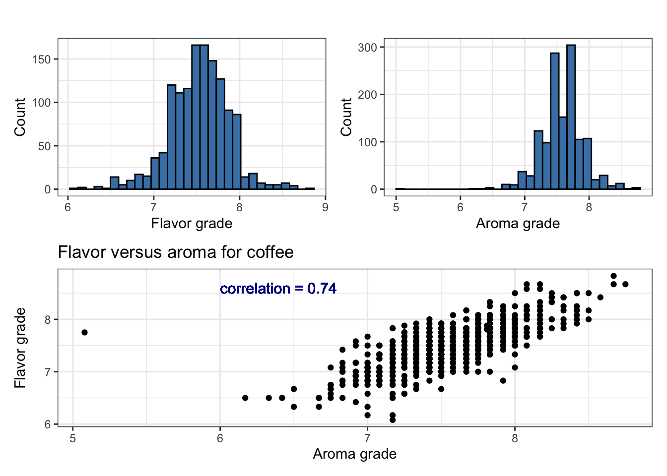
From the exploratory data analysis in Figure 6.1, we see preliminary indication of a relationship between the aroma and flavor grades. We also see there is an outlier observation that has a very low aroma grade close to 5 but a flavor grade close to the average.

Table 6.2: Linear regression model of the aroma versus flavor of coffees

term	estimate	std.error	statistic	p.value	conf.low	conf.high
(Intercept)	1.468	0.151	9.747	0	1.173	1.764
aroma	0.800	0.020	40.251	0	0.761	0.839

We use the model in Table 6.2 to describe the relationship between the aroma and flavor of coffee. For each additional point in the aroma grade, the flavor grade is expected to increase by 0.8 points, on average. From the inferential results, we conclude there is a statistically significant relationship between aroma and flavor, given p-value $\approx 0$ and the 95% confidence that does not include 0. In fact, we are 95% confident that for each additional point in the coffee grade, the flavor grade increases by 0.761 to 0.839 points, on average. In summary, coffees that smell better are expected to taste better!

We’ve made these conclusions using inferential methods introduced in Chapter 5, which rely on a set of underlying assumptions about the data. Though we are unable to check if these underlying conditions hold for the entire population, we will see in Section 6.3 how we are able to check a set of model conditions to assess whether these assumptions reasonably hold for our sample data.

As apparent in Figure 6.1, there is an outlying observation that is outside the general trend of the data, given its aroma grade is much lower than the others but its flavor grade is around the average. This is a valid data point and not the result of data entry error; therefore, we’d like to assess whether this outlier is having a noticeable impact on the estimated regression model and inferential conclusions. In Section 6.7, we will analyze a set of model diagnostics to assess the potential impact of this observation, and the impact of outliers more generally, on our results.

6.3 Model conditions

6.3.1 Assumptions for simple linear regression

Section 5.3 introduced the underlying assumptions we make about the population when doing simple linear regression. These assumptions are important, as the reliability of our interpretations and conclusions from the regression analysis rely being consistent with the assumed framework. There are various analysis questions we can answer with a simple linear regression model - describe the relationship between a response and predictor variable, predict the response given values of the predictor, and draw conclusions from simulation-based or Central Limit Theorem-based inference. As we’ll see in this chapter, we need some or all of these assumptions to hold depending on the analysis procedure.

The assumptions are based on population-level data, yet we work with sample data in practice. Therefore, we have a set of model conditions we can check using the sample data to assess the assumptions from Section 5.3.

6.3.2 Model conditions (LINE)

After fitting a simple linear regression model, we check four conditions to assess whether the data are consistent with the underlying assumptions. They are commonly referred to as LINE to help us more easily remember them. These four conditions are the following:

Linearity: There is a linear relationship between the response and predictor variables.
Independence: The residuals are independent of one another.
Normality: The distribution of the residuals is approximately normal.
Equal variance: The spread of the residuals is approximately equal for all predicted values.

After fitting the regression model, we calculate the residuals for each observation, $e_{i} = y_{i} - {\hat{y}}_{i}$ , and use the residuals to check the conditions.

The residuals, along with other observation-level statistics, can be obtained using augment() in the broom R package (Robinson, Hayes, and Couch 2023). This package is in the suite of packages that are included as part of tidymodels(Kuhn and Wickham 2020). The output produced by this function is shown in Table 6.3. This data frame includes the response and predictor variables in the regression model along with observation-level statistics, such as the residuals. The residuals (.resid) are the primary statistics of interest when checking model conditions. In a later section, we will utilize the other columns produced by augment() when we check a set of model diagnostics.

Table 6.3: First ten rows of output produced by the augment function

flavor	aroma	.fitted	.resid	.hat	.sigma	.cooksd	.std.resid
8.83	8.67	8.40415	0.42585	0.00978	0.22937	0.01715	1.86401
8.67	8.75	8.46815	0.20185	0.01114	0.22960	0.00440	0.88414
8.50	8.42	8.20415	0.29585	0.00613	0.22953	0.00515	1.29260
8.58	8.17	8.00415	0.57585	0.00342	0.22913	0.01084	2.51253
8.50	8.25	8.06815	0.43185	0.00419	0.22936	0.00747	1.88495
8.42	8.58	8.33215	0.08785	0.00836	0.22966	0.00062	0.38426
8.50	8.42	8.20415	0.29585	0.00613	0.22953	0.00515	1.29260
8.33	8.25	8.06815	0.26185	0.00419	0.22956	0.00275	1.14293
8.67	8.67	8.40415	0.26585	0.00978	0.22955	0.00668	1.16367
8.58	8.08	7.93215	0.64785	0.00268	0.22898	0.01072	2.82562

We introduce the four model conditions in order based on the LINE acronym; however, the conditions may be checked in any order.

6.3.3 Linearity

The linearity condition states that there is a linear relationship between the response and predictor variable. Though we don’t expect the relationship between the two variables to be perfectly linear, it should be linear enough that it would be reasonable to describe the relationship between the two variables using regression.

Recall from Section 6.2 that we used a scatterplot and the correlation coefficient to describe the shape and other features of the relationship between the aroma (predictor) and flavor (response). This exploratory data analysis provides an initial assessment of whether the linear regression model seems like a reasonable fit for the data. For example, if we saw a clear curve in the scatterplot or calculated a correlation coefficient close to 0, we might conclude that the proposed simple linear regression model would not sufficiently capture the relationship between the two variables and thus rethink the modeling strategy. While the exploratory data analysis can help provide initial assessment and help us thoughtfully consider our modeling approach, it should not be solely relied upon as the final assessment of whether the proposed model sufficiently captures the relationship between the two variables. We analyze the residuals for that assessment.

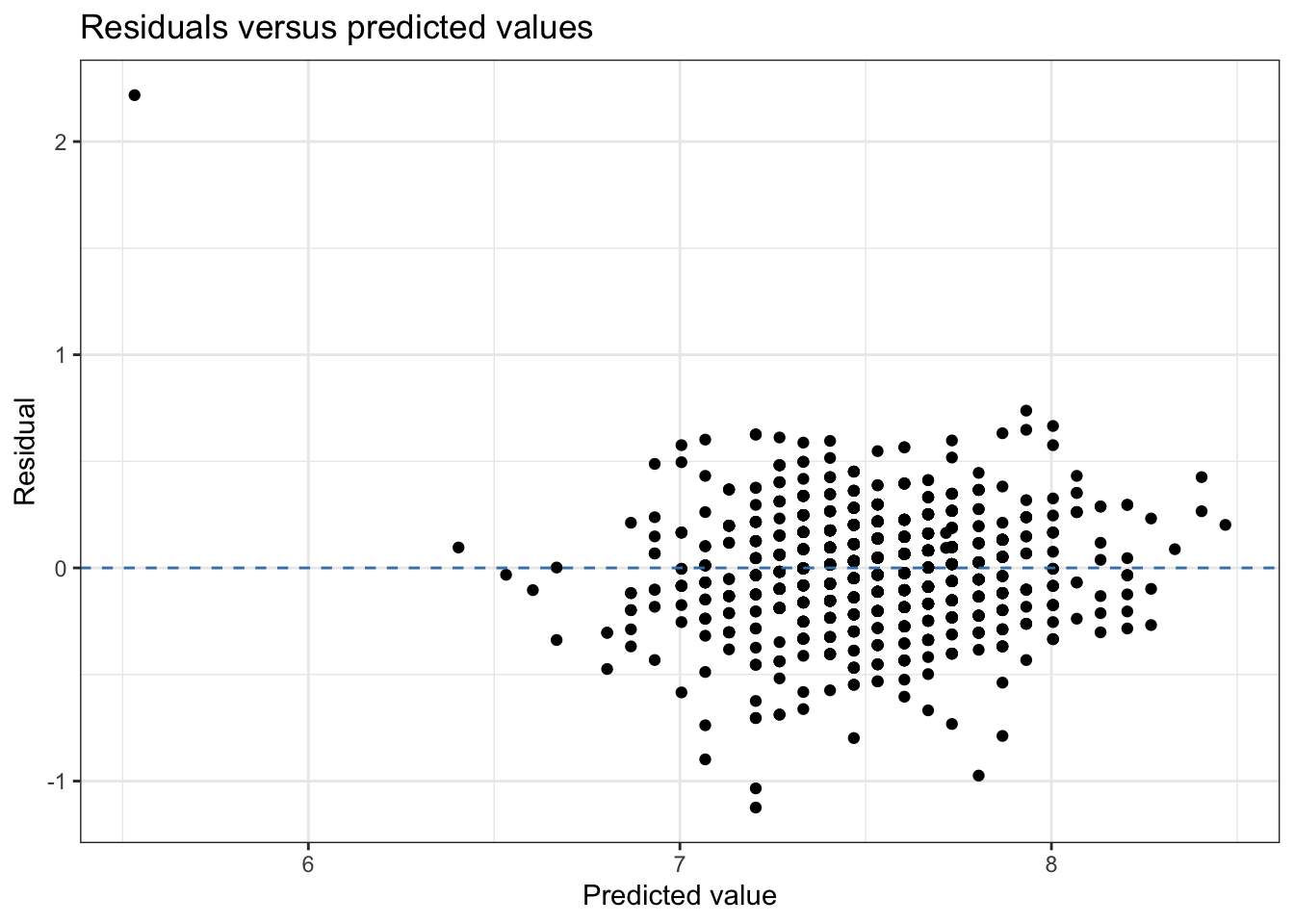
To check linearity, we make a scatterplot of the residuals (.resid) versus the predicted values (.fitted) as shown in Figure 6.2. We include a horizontal line at $y = 0$ to more easily see when the model over or under predicts.

Figure 6.2: Residuals versus predicted flavor values in coffee model

You may have noticed that this scatterplot looks very different than any of the scatterplots we’ve seen thus far in the exploratory data analysis sections in the text. Let’s break down what this plot is showing, then use it to make an assessment about the linearity condition.

When we fit a linear regression model, we are using the predictor to explain some of the variability in the response variable. Thus the residuals represent the remaining variability in the response variable that is not explained by the regression model (see Section 4.7.2 for more detail.). If the relationship between the response and predictor is linear, then we would expect the linear regression model has sufficiently captured the systematic relationship between the two variables, leaving the residuals to capture any random variability we generally expect when analyzing sample data. Let’s keep this in mind when examining the plot of the residuals versus fitted values.

We determine that the linearity condition if the residuals are randomly scattered around 0. You can assess this by asking the following:

Based on the plot, can you generally determine with great certainty whether the residual would be positive or negative for a given fitted value or range of fitted values?

If the answer is no, then the linearity condition is satisfied.
If the answer is yes, then the current linear model is not adequately capturing the relationship between the response and predictor variables. A model that incorporates information from more predictors or a different modeling modeling approach is needed (we’ll discuss some of these in later chapters!).

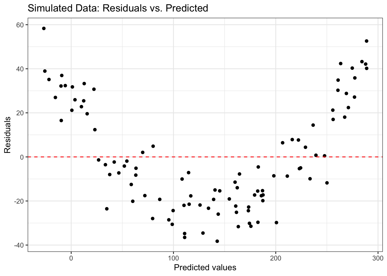
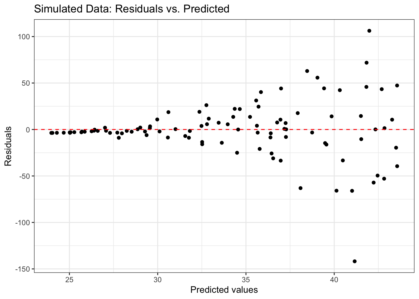
Figure 6.3 shows an example of a residual plot for simulated data in which the linearity condition is not met. There is a parabolic pattern in the plot, so the residuals are not randomly scattered around 0.

Figure 6.3: Example of violation in linearity condition. The residuals are not randomly scattered around 0.

Now let’s use the plot of residuals versus fitted values in Figure 6.2 to assess the linearity condition for the model in Table 6.2. Based on this plot, we conclude the linearity condition is satisfied. We cannot determine with great certainty whether the residual will be positive or negative for any predicted value or range of predicted values, as the points are randomly scattered around the horizontal line at $y = 0$ . Thus the linear model adequately captures the relationship between aroma and flavor grades, and the residuals capture the random variability in flavor grade due to sources other than the aroma.

6.4 What about outliers?

Notice that we made the assessment about linearity considering the range of fitted values that represents the bulk of the data. Because there is only one outlying observation with a fitted value less than 6, we are unable to determine what the random variability of the residuals would look like for fitted values in this range. Thus the presence of outliers generally does not affect our assessment about linearity.

We will discuss outliers more in-depth in Section 6.7.

6.4.1 Independence

The next condition is independence, meaning the residuals are independent of each other and that the signs of one residual do not inform the sign of other residuals. This condition is primarily checked based on the given information about the subject matter and the data collection process. This condition can be more challenging to assess, especially if we do not have much information about the data. If the condition is violated, there are two general scenarios in which the violation occurred. If neither of these apply to the data, then it is usually reasonable to conclude that the condition is satisfied.

The first scenario in which independence is often violated is due to a serial effect. This occurs when data have a chronological order or are collected over time and there is some pattern in the residuals when examining them in chronological order. If the data have a natural chronological order or were collected over time, make a scatterplot of residuals versus time. Similar to checking the linearity condition, seeing no discernible pattern in the plot indicates the independence condition is satisfied. In this case, it means that knowing something about the order in which an observation was collected does not give information about whether the model tends to over or under predict.

The second common violation independence is due to a cluster effect. This is when there are subgroups present in the data that are not accounted for by the model. To check this condition, modify the plot of the residuals versus predicted by using color, shape, faceting, or visual features to differentiate the observations by the subgroup. Similar to checking the linearity condition, we expect the residuals to be randomly scattered above and below $y = 0$ for each subgroup. If this is not the case, there is indication that subgroup should be accounted for in the model. We will talk more about strategies for dealing with violations in the model conditions in Section 6.6 and how to include categorical predictors such as subgroup in our models in Chapter 7.

6.4.2 Normality

The next condition is normality. It states that the residuals are normally distributed. Though not explicitly part of the condition, we also know that the mean of the residuals, and thus the center of the distribution, is approximately 0. This condition arises from the assumption from Section 5.3 that the distribution of the response variable, and thus the residuals, at each value of the predictor variable is normal. In practice, it would be nearly impossible to check the distribution of the response or residuals for each possible value of the predictor, so we will look at the overall distribution of the residuals to check the normality condition.

mean_resid <- mean(coffee_model_aug$.resid)
sd_resid <- sd(coffee_model_aug$.resid)

ggplot(data = coffee_model_aug, aes(x = .resid)) +
  geom_histogram(aes(y = after_stat(density)), fill = "steelblue", color = "black") +
    stat_function(
    fun = dnorm, 
    args = list(mean = mean_resid, sd = sd_resid), 
    lwd = 2, 
    color = 'red') +
  theme_bw() + 
  labs(x = "Residuals", 
       y = "", 
       title = "Distribution of residuals",
       subtitle = "with normal density curve")

Figure 6.4: The distribution of the residuals is approximately normal

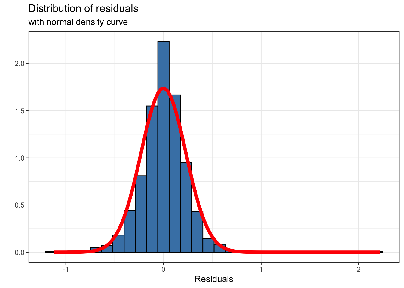
Figure 6.4 shows the distribution of the residuals along with the theoretical curve for a normal distribution that is centered at 0 the mean of the residuals, and a standard deviation of 0.229, the standard deviation of the residuals. Similar to the other conditions, we are looking for obvious departures from normality when assessing this condition. This might include strong skewness, multiple modes, large outliers, or other major departures from normality.

From Figure 6.4, we see the distribution of the residuals is approximately normal, as the shape of the histogram is unimodal and symmetric, the general shape of the normal curve. Therefore, we conclude that the normality condition is satisfied.

6.4.3 Equal variance

The last condition is equal variance, that the variability of the residuals is approximately equal for each predicted value. This condition stems from the assumption in Section 5.3 that $σ_{ϵ}^{2}$ , the variance of the distribution of the response for each value of the predictor variable does not depend on the value of the predictor (and thus does not depend on the predicted value).

To check this condition, we will go back to the plot of the residuals versus predicted values from Figure 6.2. We want to assess if the vertical spread of the residuals is approximately equal as we move along the $x$ -axis. Since we are working with sample data, we don’t expect the vertical spread of the residuals to be exactly equal as we move along the $x$ -axis (for example, there may be outliers). Therefore, similar to previous conditions, we are looking for obvious departures from equal variance to conclude that the condition is not met. Figure 6.5 shows an example using simulated data of plot of residuals versus fitted when the equal variance condition is not satisfied. Additionally, keep in mind that we are examining the vertical spread for the majority of the data, not including outliers in the assessments as shown by the dotted lines in Figure 6.6 to serve as a guide as we assess equal variance.

Figure 6.5: Example of violation in equal variance assumption. The vertical spread of the residuals increases as the predicted value increases.

Now let’s take a look at the residuals versus predicted values for the coffee ratings data.

ggplot(data = coffee_model_aug, aes(x = .fitted, y = .resid)) +
  geom_point() +
 # geom_hline(yintercept = 0, color = "steelblue", linetype = 2) +
 geom_hline(yintercept = 0.8, color = "darkcyan", linetype = 2) + 
 geom_hline(yintercept = -1, color = "darkcyan", linetype = 2) +
  theme_bw() + 
  labs(x = "Predicted value", 
       y = "Residual", 
       title = "Residuals versus predicted values")

Figure 6.6: Plot of the residuals versus predicted values. The vertical spread is approximately for each predicted value, as shown by the residuals generally falling between the two dotted lines when moving along the $x$ -axis.

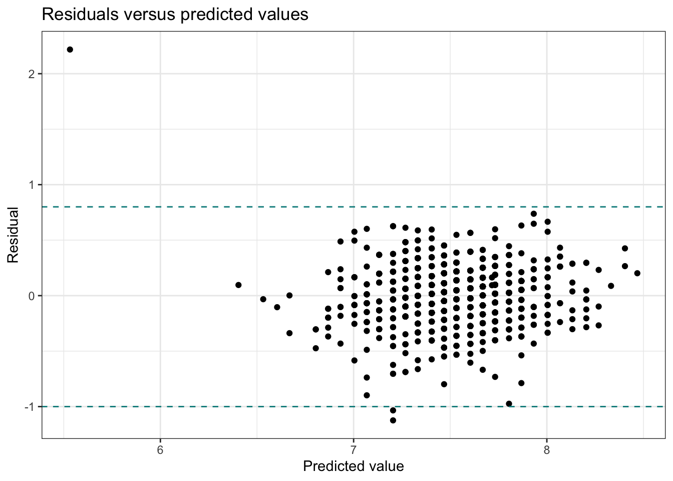
From Figure 6.6, we see that the vertical spread of the residuals is approximately equal, i.e. between the two dotted lines as we move along the $x$ -axis. Therefore, the equal variance condition is satisfied.

6.5 Recap: Checking model conditions

Linearity: Plot residuals versus predicted values. Look for points to be randomly scattered.
Independence: Use the description of the data and data collection process to assess if the observations can reasonably be treated as independent. If data are collected over time, examine plot of residuals versus time to assess potential serial effect. If unaccounted for subgroups are represented in the data, examine plot of residuals versus predicted for each subgroup.
Normality: Plot the distribution of the residuals. Look for a distribution that is approximately unimodal and symmetric.
Equal variance: Plot the residuals versus predicted values. Look for approximately equal vertical spread as you move along x-axis.

6.6 What if some (or all) conditions are not satisfied?

If all the model conditions are satisfied, we can move on to the next step in the analysis without further assessment of the conditions; however, that is often not the case in practice. The good news is we there are a variety of methods to address violations in the model conditions. Additionally, many of the analysis tasks we do are robust to violations in some of the model conditions, meaning we can still obtain reliable analysis results, even if some conditions are not satisfied.

For each model condition we will discuss the analysis tasks for which satisfying the model condition is very important and some approaches we can take to address the violations in the condition.

6.6.1 Linearity

The linearity condition is the most important condition, because the regression analysis relies on the assumption that the linear regression model adequately captures the relationship between the response and predictor variable (see Section 4.3.2). Therefore, the linearity condition must be satisfied in order for any interpretations and conclusions from the regression analysis to be useful and reliable. This means it is necessary for fitting the linear model, interpreting the slope and intercept, drawing conclusions inference conducted using simulation-based methods or the Central Limit Theorem.

If the linearity condition is not satisfied, we can ask ourselves a few questions:

Is the violation in the linearity condition due to the fact that there is, in fact, no evidence of a meaningful relationship between the response and predictor variable? In this case, reconsider if a linear regression model is the most useful way to understand these data.
Is the violation in the linearity condition because there is evidence of a meaningful relationship between the response and predictor variable; however, it is non-linear (for example, the relationship is best represented by a curve)? If this is the case, there are a few options to work with this non-linear relationship.
- Add a higher-order term, for example $x^{2}$ , in the model to capture the non-linearity of the relationship. We discuss higher-order model terms in more detail in a later section.
- Apply a transformation on the response and/or predictor variable, so there is a linear relationship between the transformed variables. Then proceed with simple linear regression using the transformed variable(s). We discuss transformations in more detail in a later section.

6.6.2 Independence

The independence condition states that the residuals are independent of one another. This assurance is most important when estimating variability about the line or variability in the estimated regression coefficients when doing statistical inference. If the independence condition is not satisfied and some residuals are correlated with one another, then our procedures may underestimate the true variability about the regression line and ultimately the variability in the estimated regression coefficients . This is due to the fact that each observation is not fully contributing new information, because there is some correlation between two or more observations. Thus the effective sample size, or how many observations independently provide information, is smaller than the true sample size $n$ . This could result in misleading inferential conclusions, such as concluding there is a linear relationship between the response and predictor variable, when in fact there is not such a relationship.

If the independence condition is not met, more advanced statistical methods would be required to properly deal with the correlated residuals. These methods are beyond the scope of this book, but you can learn more about these methods called multilevel models or hierarchical models in texts such as Roback and Legler (2021).

If we observe some pattern in the residuals based on subgroup, then there are two approaches to address it. The first is creating a separate model for each subgroup. The primary disadvantage to this approach is that we may have a different estimate for the slope and intercept for each subgroup, and thus it may be more difficult to draw overall conclusions about the relationship between the response and predictor variables.

The second option is to fit a model that includes the subgroup as a predictor. This will allow us to account for differences by subgroup while maintaining a single model that makes it easier to draw overall conclusions. This type of model is called a multiple linear regression model, because it includes more than one predictor variable. We will introduce these models more in detail in Chapter 7.

If the violations in the independence condition are not addressed, we must use caution when drawing conclusions from the model or calculating predictions given the systematic under or over prediction by subgroup. In this case, we should consider if the model can be used to produce the type of valuable insights we intend.

6.6.3 Normality

By the Central Limit Theorem, we know the distribution of the estimate slope (the statistic of interest) is normal when the sample size is sufficiently large (see Section 5.9 for more details), regardless of the distribution of the original data. Therefore, when the sample size is “large enough”, we can be confident that the distribution of the estimated slope ${\hat{β}}_{1}$ is normal, even if the residuals (and thus the response variable) do not follow a normal distribution.

A common threshold for a “large enough” sample size is 30. This means if the sample has at least 30 observations (which is often the case for modern data sets!), we can use all the methods we’ve discussed to fit a simple linear regression model and draw conclusions from inference, even if the residuals are not normally distributed. Thus the inferential methods based on the Central Limit Theorem are considered robust to violations in the normality assumption, because we can feel confident about the conclusions from the inferential procedures even if the normality condition is not satisfied (given $n > 30$ ). One note of caution is that if the sample size is very close to 30, then the inferential methods based on the Central Limit Theorem are not robust to major departures form normality such as extreme skewness or outliers.

Recall from Section 5.4 the objective of simulation-based inference is to use the data to generate the sample distribution. Therefore, we do not make any assumptions about the sampling distribution of the estimated slopes. Because there are no assumptions about the sampling distribution, the normality condition is not required for simulation-based inferential procedures.

Using 30 as a threshold

Thirty should not be treated as an absolute threshold. In other words, we should not treat data with a sample size of 29 materially different from data with a sample size of 31.
What if you have a small sample size?
- The distribution of the residuals should not have large departures from normality, in order to have reliable conclusions from the CLT-based inferential results.
- You can conduct simulation-based inference, because these methods do not make any assumptions about the sampling distribution of ${\hat{β}}_{1}$ .

6.6.4 Equal variance

The equal variance condition is as assessment of whether the distribution of the residuals is approximately equal for each value of the predictor variable. This is equivalent to the distribution of the response about the line for each predictor variable. The regression standard error ${\hat{σ}}_{ϵ}$ is the estimated value of this variability about the line, and it is the assumed to be the same for all values of the predictor (see Section 5.3 for more detail). When conducting inference based on the Central Limit Theorem, this regression standard error is used to calculate $S E_{{\hat{β}}_{1}}$ , the estimated standard error for the estimated slopes. Thus similar to violations in the independence condition, if the variability about the regression line is not equal for all values of the predictor, the regression standard error will not be accurate and thus the standard error of the slope, our estimate of the sampling variability in this statistic will be inaccurate as well. The calculation of the confidence interval and test statistic for hypothesis testing both use $S E_{{\hat{β}}_{1}}$ , so these values will likely be inaccurate as well. Therefore, we should approach conclusions from the inferential procedures with caution if the equal variance condition is not met.

Similar to the normality condition, the equal variance condition is not required for simulation-based inference, because $S E_{{\hat{β}}_{1}}$ is estimated from the sampling distribution simulated from the data.

There are approaches for handling violations in the equal variance condition. These approaches typically involve performing a transformation on the response variable. We will discuss these further in a later chapter.

6.6.5 Recap

Table 6.4 provides a summary of the model conditions and whether they must be satisfied to reliably conduct each modeling task.

Table 6.4: Summary of when model conditions must be satisfied

Model condition	Interpret ${\hat{β}}_{1}$	Simulation-based inference for ${\hat{β}}_{1}$	Inference based on Central Limit Theorem for ${\hat{β}}_{1}$
Linearity	Important	Important	Important
Independence	Important	Important	Important
Normality	Not need	Not needed	Not needed if $n > 30$ Important if $n < 30$
Equal variance	Not needed	Not needed	Important

So far we have discussed the model conditions to assess whether the assumptions for simple linear regression from Section 5.3 reasonably hold true for our data. We have not, however, dealt with the presence of outliers in the data and the potential impact (or “influence”) they may have on the regression model. In the next section, we discuss measures we can use to identify and assess the potential impact of such observations.

6.7 Model diagnostics

One challenge that may arise when doing regression analysis (or really any type of data analysis) is how to handle outliers in the data. Because we are focused on the linear relationship between two (and eventually three or more) variables, there are multiple ways in which the outliers may show up in our analysis:

Outliers in the value of the predictor variable
Outliers in the value of the response variable
Outliers outside the general pattern of the relationship between the response and predictor variables

A single observation could fall into multiple categories. For example look at the outlier identified in Figure 6.1. This observation is around the center of the distribution for the response variable flavor_grade but has low outlying value in terms of the predictor aroma_grade. Therefore, it is an outlier as described by categories (1) and (3) above.

In addition to identifying outliers, we also want to assess whether the outliers are making an out-sized impact on the analysis. We have a set of model diagnostics to assess if there are observations in the data that fall into one or more of these outlier scenarios, and more importantly, if any such outlying observations have an out-sized impact on the regression model.

6.7.1 Influential points

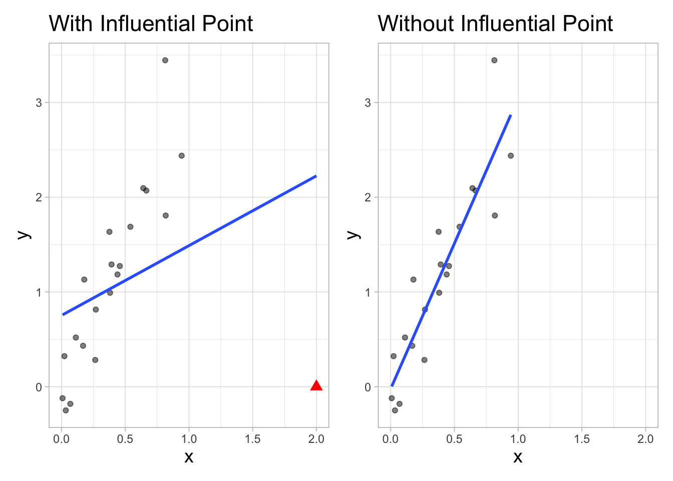
An observation is considered an influential point if the estimated regression coefficients noticeably differ when the point is included in the model fit versus when it is not. Figure 6.7 illustrates the potential impact an influential point can have on the estimated regression line. Additionally, influential points can affect $S E_{{\hat{β}}_{1}}$ , estimated standard error of the slope, which can result in unreliable inference conclusions as described earlier.

Figure 6.7: Simulated data showing the effect of an infulential point denoted as a red triangle. The slope of the line changes when the influential point is removed from the data set.

Sometimes potential influential points can be identified in a scatterplot of the response versus predictor variable in the exploratory data analysis. In the EDA, we have called out these points as being outliers, as they are typically outside of the general trend of the relationship between the two variables. Identifying these points from the EDA can become more difficult, however, when there are multiple predictor variables (see Chapter 7). Therefore, we will use a set of model diagnostics to identify observations that are outliers and perhaps more importantly, those that are influential points.

There are three diagnostic measures to identify outliers and influential points:

Leverage: identify observations that are outliers in the values of the predictor
Standardized residuals: identify observations that are outliers in the value of the response
Cook’s distance: identify observations that are influential points (a combination of leverage and standardized residuals)

Ultimately, we are most interested in examining Cook’s distance, because it provides the indication about each observation’s impact on the regression analysis. Cook’s distance takes into account information gleaned from leverage and standardized residuals, so we will introduce these diagnostics first, then discuss Cook’s distance in detail.

6.7.2 Leverage

The leverage of the $i^{t h}$ observation is a measure of the distance between its value of the predictor, $x_{i}$ , the average value of the predictor across all $n$ observations, $\bar{x} = \frac{1}{n} \sum_{j = 1}^{n} x_{j}$ .

When doing simple linear regression, an observation’s leverage, denoted $h_{i}$ , is calculated using Equation 6.1.

$\begin{matrix} (6.1) & h_{i} = \frac{1}{n} + \frac{(x_{i} - \bar{x})^{2}}{\sum_{j = 1}^{n} (x_{j} - \bar{x})^{2}} \end{matrix}$

The values of the leverage are between $\frac{1}{n}$ and 1 for each observation in the data set, and the average value of leverage across all $n$ observations is $\frac{(p + 1)}{n}$ , where $p$ is the number of predictors in the model. In simple linear regression $p = 1$ , thus the average leverage is $\frac{2}{n}$ .

An observation is considered to have large leverage if it’s leverage is greater than $\frac{2 (p + 1)}{n}$ , i.e., greater than $\frac{2 \times 2}{n}$ for simple linear regression. This means that an observation is considered to have large leverage if its value of leverage is greater than twice the average value of leverage for the observations in the data set.

Important

Leverage only depends on the values of the predictor variable(s). It does not depend on values of the response.

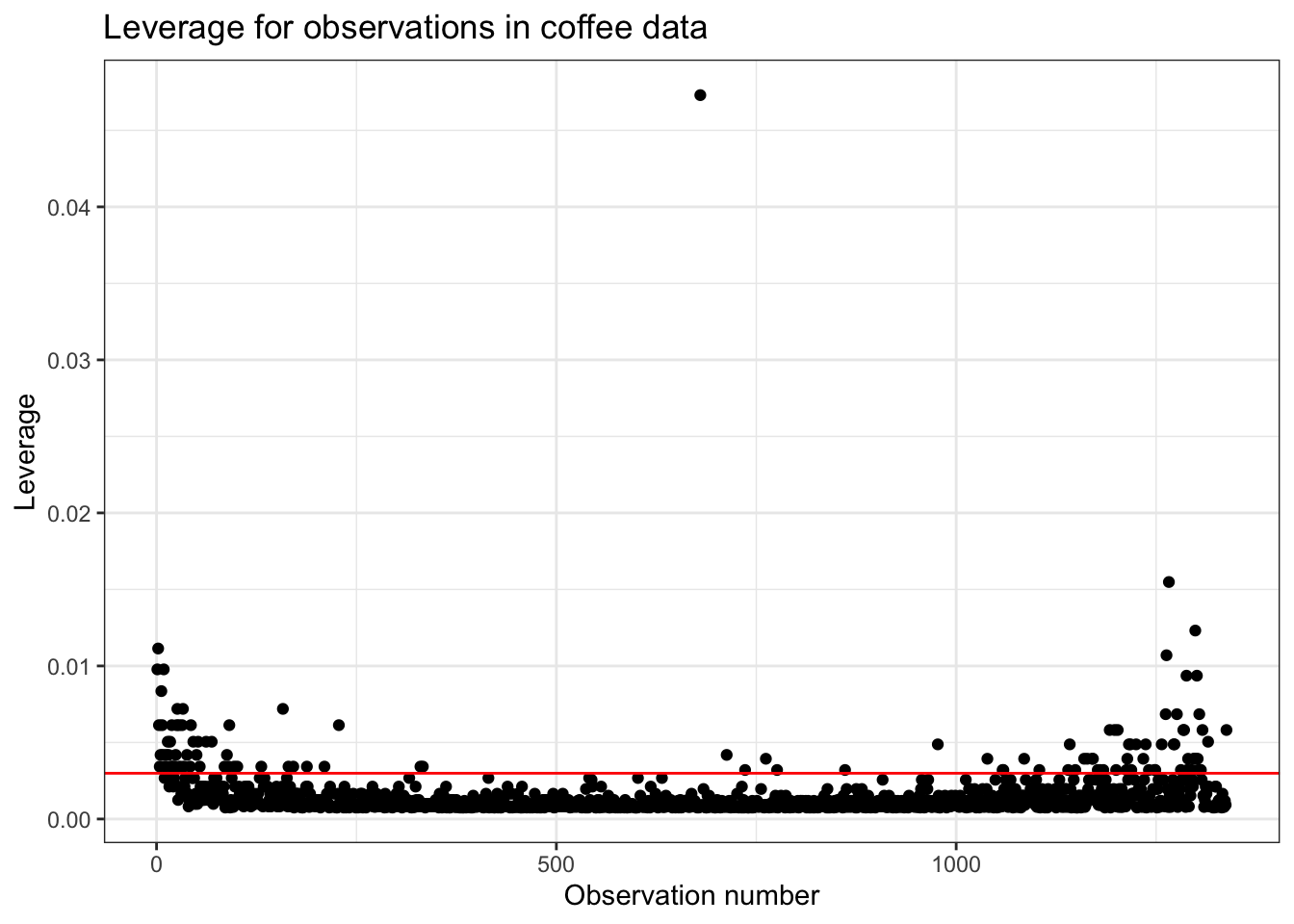
Let’s take a look at the leverage for the observations in the coffee_ratings data set. There are 1338 observations in the data and one predictor variable. Therefore, the threshold for identifying observations with large leverage is $\frac{2 \times 2}{16} =$ 0.003.

Figure 6.8 is a visualization of the leverage for each observation in the data set. The red, horizontal dotted line marks the threshold for identifying points as having large leverage. There are 114 observations that have large leverage.

Figure 6.8: Leverage for observations in the coffee

Your turn!

There are 114 observations that have large values for the leverage. What does it mean for an observation to have “large leverage” in the context of the coffee data?

Let’s take a look at the observations with the largest values of of leverage to get a better understanding about which points may be large leverage.

Table 6.5: Observations with the top five highest values for leverage

.hat	aroma	flavor
0.047	5.08	7.75
0.015	6.17	6.50
0.012	6.33	6.50
0.011	8.75	8.67
0.011	6.42	6.50

Recall that the leverage only depends on the values of the predictor variable, so we only need to consider aroma to better understand why these points are large leverage. As we saw in Section 6.2, the average aroma grade in the data set is 7.572 points and the standard deviation is 0.316 . The observations with the largest values of leverage have aroma grades that are either much higher (e.g., 8.75) or much lower (e.g., 5.08) than the average. Thus the large leverage points includes coffees that both smell much better and perhaps must worse than the rest of the coffees in the data.

Even when we identify points with large leverage, we still want to understand how these points are (or are not) influencing the model results. Thus, knowing an observation has large leverage is not enough to warrant any specific action. We’ll examine Cook’s distance to determine if it is influential in the model and discuss approaches to deal with influential points in Section 6.7.6 .

6.7.3 Standardized residuals

In #sec-slr-estimation we introduced residuals, the difference between the observed and predicted response ( $e_{i} = y_{i} - {\hat{y}}_{i}$ ). The residual is an indication of how well the regression model predicted the value of the response for a given observation, and one reason the model may predict poorly for an observation is because it has an observed value of the response that is much different than the rest of the data. Therefore residuals can be used to identify observations that are outliers based on Scenario 2. We will examine the magnitude of the residuals $| e_{i} |$ to identify such points, because residuals can be positive (mode underpredicted) or negative (model overpredicted).

The residuals have the same units as the response variable, so what is considered a residual with large magnitude depends on the scale and range of the response variable. This means what is considered a “large” residuals can be different for every analysis. We can address this by instead examining standardized residuals, defined as the residual divided by its standard error. Equation 6.2 shows the formula to calculate the standardized residual for the $i^{t h}$ observation.

$\begin{matrix} (6.2) & s t d . r e s i d_{i} = \frac{e_{i}}{S E_{e_{i}}} = \frac{e_{i}}{{\hat{σ}}_{ϵ} \sqrt{1 - h_{i}}} \end{matrix}$

The residuals for every analysis are now on the same scale. Thus, we can use a common threshold to determine residuals that are considered to have large magnitude. An observation is an outlier in the response if it its standardized residual has a magnitude greater than two, $| s t d . r e s i d_{i} | > 2$ ( $s t d . r e s i d_{i} < - 2 or s t d . r e s i d_{i} > 2$ ).

Why is the threshold 2?

Recall that one assumption for linear regression is that the residuals are normally distributed and centered at 0 (see Section 5.3). This means the standardized residuals are normally distributed with mean of 0 and standard deviation of 1, $N (0, 1)$ . In a standard normal distribution, we expect about 95% of the observations to have values between -2 and 2. By setting 2 as the threshold, we are essentially identifying the 5% of observations with the most extreme (high and low) residuals.

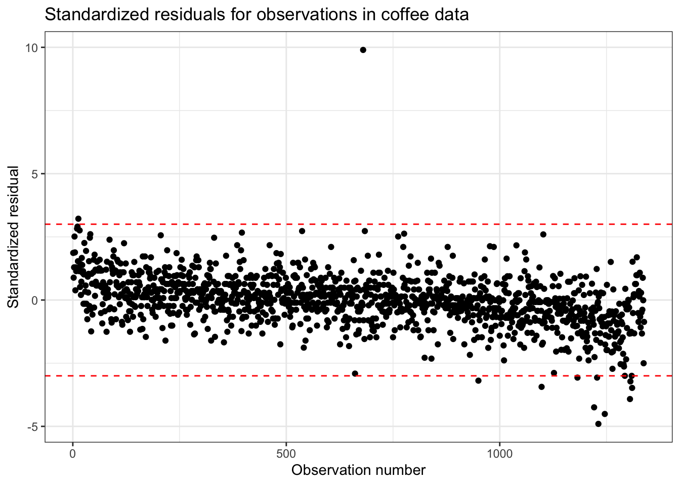
If you have a lot of observations, it may not be practical to closely examine the approximately 5% of observations that were identified as potential outliers. Thus you may use a more restrictive threshold, e.g., $| s t d . r e s i d_{i} | > 3$ (or higher) to identify points worth more close examination or focus on those that are identified as influential points by Cook’s distance.

Figure 6.9: Standardized residuals from model of coffee flavor versus aroma grade

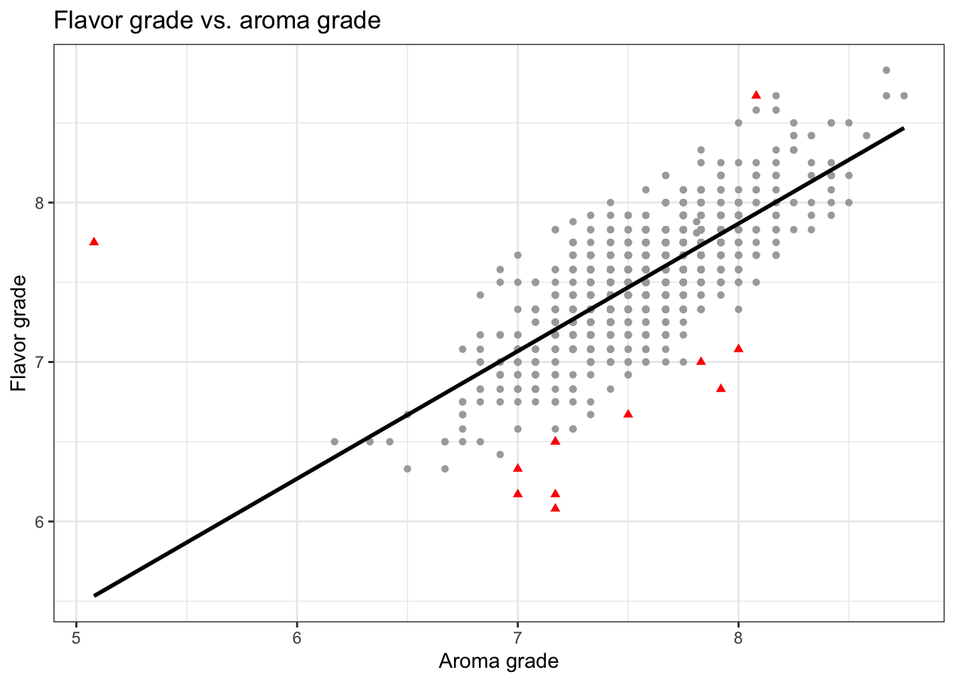
Figure 6.9 shows 12 observations with large magnitude residuals based on the threshold $\pm 3$ . This includes observations that have positive residuals with large magnitude (indicating the model greatly underpredicted) and observations with negative residuals with large magnitude (indicating the model greatly overpredicted).

These five observations with the largest magnitude residuals are shown in Table 6.6.

Table 6.6: Observations with large magnitude residuals

aroma	flavor	.fitted	.std.resid
5.08	7.75	5.532	9.897
7.17	6.08	7.204	-4.901
7.17	6.17	7.204	-4.509
7.92	6.83	7.804	-4.247
7.00	6.17	7.068	-3.918

We see from Table 6.6 and Figure 6.10 that these observations have flavor ratings that are lower than would be expected from the model based on their aroma ratings. The exception is the observation with the largest magnitude standardized residual that has a higher actual flavor rating than the model predicts based on its very low aroma rating.

Figure 6.10: Flavor grade versus aroma grade. Points marked with a red triangle are the observations with large standardized residuals with magnitude > 3.

Use standardized residuals for model conditions

We can use a plot of standardized residuals versus predicted values such as the one in Figure 6.9 to check the linearity and constant variance conditions from Section 6.3. Therefore, when doing an analysis, use the plot of standardized residuals, so you can check the model conditions and identify outliers using the same plot.

As with observations that have large leverage, we want to assess whether these points have out-sized influence on the model coefficients to help determine how to deal with these outliers (or if we need to do anything at all). To do so, we will look at the last diagnostic, Cook’s distance.

6.7.4 Cook’s distance

At this point we have introduced a diagnostic to identify outliers in the predictor variable (leverage) and one to identify outliers in the response variable (standardized residuals). Now we will use a single measure that combines information we glean from the leverage and standardized residuals to help identify potential influential points. This measure is called Cook’s distance.

Cook’s distance is a measure of an observation’s overall impact on the estimated model coefficients. One can think of it as a measure of how much the model coefficients change if a given observation is removed. In Equation 6.3, we see that Cook’s distance takes into account an observation’s leverage, $h_{i}$ , the standardized residuals, $s t d . r e s i d_{i}$ , and the number of predictors in the model, $p$ ( $p = 1$ for simple linear regression).

$\begin{matrix} (6.3) & D_{i} = \frac{1}{p} (s t d . r e s i d_{i})^{2} (\frac{h_{i}}{1 - h_{i}}) \end{matrix}$

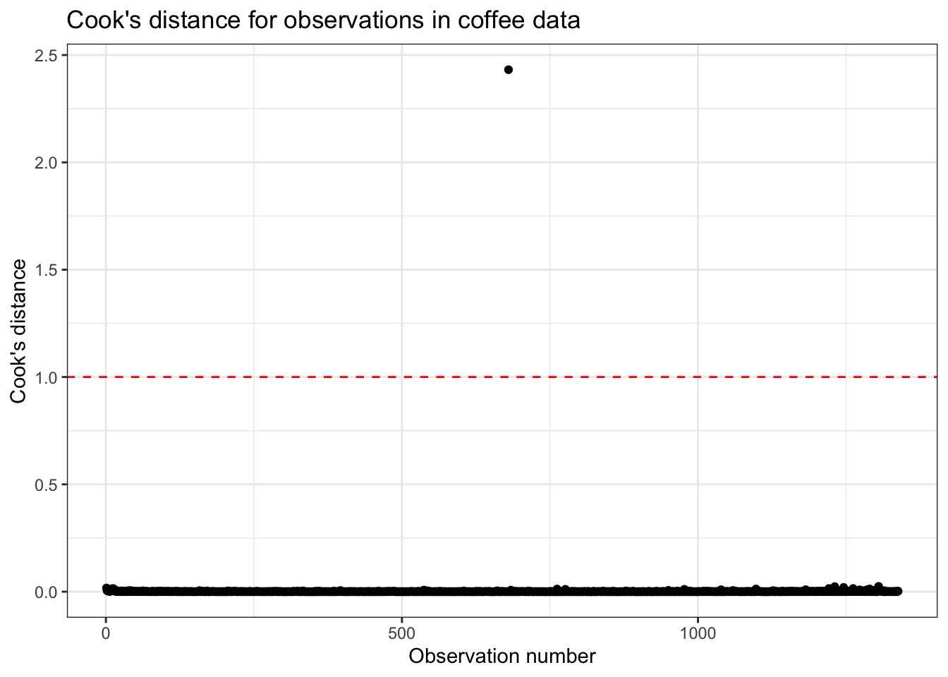
As with leverage and standardized residuals, there are thresholds we can use to determine if a point is potentially influential. A commonly used threshold is 1. If an observation has a Cook’s distance greater than 1, $D_{i} > 1$ , it is considered an influential point and is worth closer examination given its potential influence on the model.

Figure 6.11: Cook’s distance for coffee_ratings data set

Figure 6.11 shows the values of Cook’s distance for the observations in the data set. It includes a horizontal line at 1 marking the threshold for determining if an observation is influential. There is one observation in the data that has a value of Cook’s distance greater than 1; its value is 2.432.

6.7.5 Impact of influential points

To better understand the impact of influential points, let’s take a look at our model fit with and without the influential observation.

Table 6.7: Estimated model coefficients for model with and without influential observation

Term	With Influential Point	Without Influential Point
(Intercept)	1.468	1.137
aroma	0.800	0.843

We see in Table 6.7 that the estimates for the intercept and effect of aroma changed when the influential point was removed. Therefore, it is now our task as the data scientist to determine how to best proceed given the influential point.

6.7.6 How to handle outliers

You can use all the model diagnostics we’ve presented - leverage, standardized residuals, and Cook’s distance - to identify observations that are outliers and those that are also influential points. Below are general strategies for dealing with outliers.

6.7.6.1 Outlier based on predictor

If an observation is an outlier based on the predictor variable, first consider if it is the result of a data entry error that can be fixed. If not, one option is to remove this observation from the analysis, particularly if the outlier is an influential point or a result of a data entry error. Doing so limits the scope of the conclusions that can be drawn from the analysis and the range of values for which the model can be used for prediction, because removing the outlying observation narrows the range of possible values for the predictor. If you take this approach, it is important to mention it as you write up and present results. Additionally, you will need to be careful not to extrapolate if using the model for prediction.

The influential point identified in Section 6.7.4 is an outlier because it has a value of the predictor much lower than the rest of the data. Therefore, we could remove this observation and thus limit the scope of the analysis to coffee that has an aroma rating of 6 or higher. We can also keep this observation in the analysis and thus have some information about coffees with aroma ratings less than 6. Given there is a single observation with a rating less than 6, however, conclusions about coffees with low coffee ratings should be made caution.

6.7.6.2 Outlier based on response

If the observation is an outlier based on the value of the response variable, first consider if it is the result of a data entry error. If it is not and the value of the predictor is within the range of the other observations in the data, the observation should not be removed from the analysis. Removing the observation could result in taking out useful information for understanding the relationship between the response and predictor variable.

If the outlier is influential, one approach is to build the model with and without the influential point, then compare the estimated values and inference for the model coefficients. Another approach is to transform the response variable to reduce the effect of outliers (more on transformations in an upcoming chapter ). A last approach is to collect more data, so the model information can be informed by more observations; however, collecting more data is often not feasible in practice.

6.8 Modeling in practice

In this chapter, we have introduced a set of model conditions and diagnostics to assess how well the model fits the data and satisfies the assumptions for linear regression. Now we’ll conclude the chapter by discussing how we might incorporate these tools in practice.

Exploratory data analysis (EDA): Start every regression analysis with some exploratory data analysis, as in Section 6.2 . The EDA will help you better understand the data, particularly the variables that will be used for the regression model. Through the EDA you may also notice points that stand out as potential outliers and potential influential points that may be of interest for further exploration. The EDA is can help you gain valuable insights about the data; however, it cannot be used alone to confirm whether the model is a good fit or confirm if a point is influential. We need the model conditions and diagnostics to make such a robust assessment. The EDA is important, however, to help us determine the best analysis approach and to understand the data enough to more fully understand the model interpretations and influential conclusions.
Model fitting: Fit the regression model.
Model conditions and diagnostics: Check the model conditions (LINE) to assess whether the model is a good fit for the data.

Then, check Cook’s distance to determine if there are potential influential points in the data.
- If there are influential points, check the leverage and standardized residuals to try to understand why these points are influential. Use this information, along with the analysis objective and subject matter expertise, to determine how to best proceed with the dealing with these points.
- If there are no influential points, you can examine the leverage and standardized residuals for a deeper understanding of the data; however, no further action is needed in terms of refitting the model.
Make any adjustments as needed based on the model conditions and diagnostics.

[Note: Steps 2 and 3 is typically an iterative process until you find the model that is the best fit for the data.]
Prediction and inference: Once you have finalized your model and are satisfied with the results of the model conditions and diagnostics, then you can use the model for prediction and inference to answer your analysis questions.
Summarize conclusions: Once you have your final inferential results and predictions, summarize your overall conclusions in a way that can be easily understood by the intended audience.

6.9 Looking ahead

Thus far, we have discussed simple linear regression where we use one predictor variable to understand variability in the response. In the next chapter, we will extend on what we know about simple linear regression, as we discuss multiple linear regression, modeling with two or more predictors.